Linear Search vs Binary Search: Finding Data Efficiently

Searching is one of the most fundamental operations in computer science.

Almost every application needs to find something:

• Find a user by ID
• Find a product by SKU
• Find a contact by name
• Find a file
• Find a number in an array
• Find a record in a database
• Find a page in an index

At first, searching sounds simple:

"Just look for the thing."

But how you search can make an enormous difference.

Imagine searching through 10 items.

No big deal.

Now imagine searching through:

10,000 items
1,000,000 items
100,000,000 items

Suddenly, the algorithm matters.

In this article, we'll learn two foundational searching algorithms:

1. Linear Search
2. Binary Search

We'll understand how they work, write pseudocode, implement them, analyze their complexity, and discover one of the most important ideas in algorithms:

Reducing the search space.

What Is a Searching Algorithm?

A searching algorithm is a method used to determine whether a particular value exists in a collection of data and, depending on the algorithm, where it is located.

Suppose we have:

[10, 25, 37, 42, 58, 63, 79]

and we want to find:

42

A searching algorithm needs to answer:

Does 42 exist?
Where is 42?

If it exists at index 3, we might return:

3

If it doesn't exist, we might return:

-1

The Two Searching Strategies

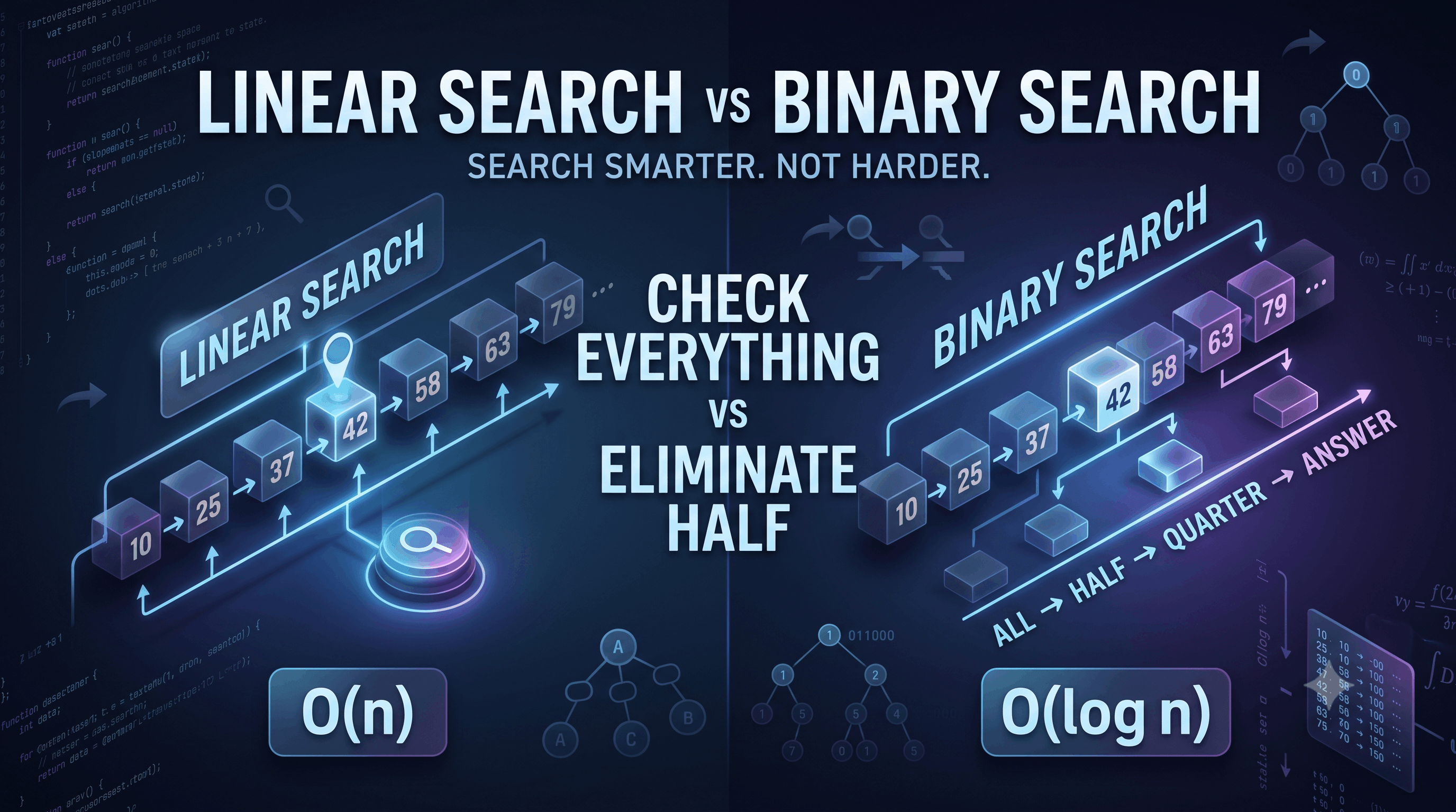
At a high level:

Linear Search

Check elements one by one.

10 → 25 → 37 → 42

Binary Search

Repeatedly eliminate half of the remaining possibilities.

[10 25 37 | 42 58 63 79]
              ↑
           middle

This fundamental difference gives them very different performance characteristics.

Part 1: Linear Search

Linear Search is the simplest searching algorithm.

The idea is straightforward:

Start at the beginning and check each element until you find the target.

Suppose we have:

[15, 28, 41, 53, 67, 82]

Target:

53

We search:

15 ❌
28 ❌
41 ❌
53 ✅

We found it.

Linear Search Algorithm

The algorithm is:

1. Start from the first element.
2. Compare it with the target.
3. If it matches, return its position.
4. Otherwise, move to the next element.
5. Repeat until the target is found or the collection ends.
6. If the target is not found, return "Not Found".

Linear Search Pseudocode

START

INPUT array
INPUT target

FOR i = 0 TO length(array) - 1

    IF array[i] = target
        RETURN i
    END IF

END FOR

RETURN -1

END

Simple.

No sorting is required.

No special data structure is required.

Linear Search Example

Consider:

numbers = [12, 45, 7, 89, 23]
target = 89

The algorithm performs:

12 == 89? → No
45 == 89? → No
7  == 89? → No
89 == 89? → Yes

Result:

index = 3

Linear Search in Python

def linear_search(numbers, target):

    for i in range(len(numbers)):

        if numbers[i] == target:
            return i

    return -1

Usage:

numbers = [12, 45, 7, 89, 23]

result = linear_search(numbers, 89)

print(result)

Output:

3

Linear Search in JavaScript

function linearSearch(numbers, target) {

    for (let i = 0; i < numbers.length; i++) {

        if (numbers[i] === target) {
            return i;
        }
    }

    return -1;
}

The logic remains the same.

Only the programming syntax changes.

Time Complexity of Linear Search

Suppose there are n elements.

In the worst case, we might inspect every element.

Therefore:

Time Complexity = O(n)

Best Case

What if the target is the first element?

[50, 20, 30, 40, 60]
 ↑
target

We find it immediately.

Best case:

O(1)

Worst Case

What if the target is the last element?

[10, 20, 30, 40, 50]
                ↑
              target

We check every element.

Worst case:

O(n)

Target Doesn't Exist

What if:

[10, 20, 30, 40, 50]

and target is:

99

We check everything:

10 ❌
20 ❌
30 ❌
40 ❌
50 ❌

Again:

O(n)

Space Complexity

Our implementation only uses a few variables.

We don't create another array.

Therefore:

Auxiliary Space = O(1)

So Linear Search has:

Best Time:   O(1)
Worst Time:  O(n)
Space:       O(1)

When Is Linear Search Useful?

Linear Search is actually a very useful algorithm.

Use it when:

• The dataset is small.
• The data isn't sorted.
• You only need occasional searches.
• Simplicity matters.
• You don't want preprocessing.
• The collection doesn't support efficient random access.

It's easy to implement and doesn't require the data to be sorted.

The Limitation of Linear Search

The problem is scalability.

Suppose we have:

n = 1,000,000

In the worst case, Linear Search may inspect:

1,000,000 elements

Now imagine:

n = 1,000,000,000

The amount of work becomes enormous.

Can we do better?

Yes.

That's where Binary Search enters.

Part 2: Binary Search

Binary Search uses a completely different strategy.

Instead of checking every element:

Check the middle and eliminate half the search space.

But there is an important requirement:

The data must be sorted.

For example:

[10, 20, 30, 40, 50, 60, 70]

Target:

60

Start by checking the middle:

[10, 20, 30, 40, 50, 60, 70]
             ↑
            40

Is:

40 == 60?

No.

Since the array is sorted and:

60 > 40

we know that everything before 40 can be ignored.

Remaining:

[50, 60, 70]

We check the middle again:

[50, 60, 70]
     ↑
    60

Found it.

The Key Idea Behind Binary Search

Binary Search doesn't ask:

"Which element should I check next?"

It asks:

"Which half can I completely eliminate?"

That's the power of Binary Search.

Binary Search Step by Step

Suppose:

[5, 10, 15, 20, 25, 30, 35, 40]

Target:

35

Step 1

Check middle:

20

Target is larger.

Eliminate:

[5, 10, 15, 20]

Remaining:

[25, 30, 35, 40]

Step 2

Middle of remaining section:

30

Target is larger.

Remaining:

[35, 40]

Step 3

Check:

35

Found.

Visualizing Binary Search

Original:

[ 5  10  15  20  25  30  35  40 ]
                ↑
              middle

Target = 35

20 < 35
↓
Eliminate left half

[ 25  30  35  40 ]
          ↑
        middle

30 < 35
↓
Eliminate left half

[ 35  40 ]
   ↑
target found

Instead of checking eight elements, we found the target after only a few comparisons.

Binary Search Pseudocode

START

INPUT sorted_array
INPUT target

left = 0
right = length(sorted_array) - 1

WHILE left <= right

    middle = (left + right) / 2

    IF sorted_array[middle] = target
        RETURN middle

    ELSE IF sorted_array[middle] < target
        left = middle + 1

    ELSE
        right = middle - 1

    END IF

END WHILE

RETURN -1

END

This is one of the most important pseudocode patterns in DSA.

Binary Search in Python

def binary_search(numbers, target):

    left = 0
    right = len(numbers) - 1

    while left <= right:

        middle = (left + right) // 2

        if numbers[middle] == target:
            return middle

        elif numbers[middle] < target:
            left = middle + 1

        else:
            right = middle - 1

    return -1

Example:

numbers = [5, 10, 15, 20, 25, 30, 35, 40]

result = binary_search(numbers, 35)

print(result)

Output:

6

Why Must Binary Search Use Sorted Data?

This is extremely important.

Suppose we have:

[40, 10, 70, 20, 50, 30, 60]

Target:

50

If we inspect the middle:

20

we cannot conclude whether 50 is on the left or right.

The data isn't ordered.

We can't safely eliminate half the elements.

Therefore:

Binary Search relies on ordering to eliminate possibilities.

Without that property, the algorithm doesn't work correctly.

Binary Search Complexity

Each step eliminates approximately half of the remaining search space.

Suppose:

n = 16

After each step:

16
 ↓
8
 ↓
4
 ↓
2
 ↓
1

Only about:

log₂(16) = 4

halving steps are needed.

Therefore:

Time Complexity = O(log n)

Linear Search vs Binary Search

Here's the fundamental comparison:

A Million Elements

Imagine:

n = 1,000,000

Linear Search

Worst case:

~1,000,000 checks

Binary Search

Approximately:

log₂(1,000,000) ≈ 20

halving steps.

That difference is extraordinary.

But There's a Catch

You might think:

"Why don't we always use Binary Search?"

Because sorting isn't free.

Suppose your data is initially:

[40, 10, 80, 20, 50]

Before Binary Search can be used, we need sorted data:

[10, 20, 40, 50, 80]

Sorting itself takes time.

For example, an efficient comparison-based sorting algorithm may take approximately:

O(n log n)

So whether sorting is worthwhile depends on how often you're going to search.

One Search vs Many Searches

Suppose you have 10 items and need to search once.

Sorting first probably isn't worth it.

But imagine:

1,000,000 records
+
1,000,000 searches

Maintaining sorted/indexed data can be extremely valuable.

This is a common engineering trade-off:

Preprocessing Cost
       ↓
Better Query Performance

A Real-World Example

Imagine an online store has millions of products.

A customer searches:

"wireless headphones"

The system can't simply scan every product every time and expect unlimited scalability.

Real production systems use more sophisticated approaches involving:

• Database indexes
• Search indexes
• Caching
• Inverted indexes
• Ranking algorithms
• Specialized search engines

But the fundamental idea remains:

Organize data so that you don't have to inspect everything.

Binary Search teaches exactly this mindset.

Binary Search in Databases

Database indexes often use tree-based structures rather than literally running the textbook Binary Search algorithm over an array.

For example, database systems commonly use structures such as B-trees and related variants.

The important conceptual connection is:

Organized data
     ↓
Efficient navigation
     ↓
Avoid scanning everything

This is why understanding basic algorithms helps you understand real software systems.

The Search Space Concept

One of the most valuable ideas from Binary Search is the concept of a search space.

Suppose:

Search Space = 1,000,000 possibilities

Linear Search:

1,000,000
 ↓
999,999
 ↓
999,998
 ↓
...

Binary Search:

1,000,000
     ↓
500,000
     ↓
250,000
     ↓
125,000
     ↓
...
     ↓
1

The second approach destroys the search space much faster.

This idea appears in many advanced algorithms.

Binary Search Is More Than Searching Arrays

This is a fascinating point.

Binary Search can be used when you can define:

1. An ordered search space
2. A way to determine which side contains the answer

For example, sometimes you don't search for a specific value.

Instead, you search for the minimum possible answer or maximum possible answer.

This technique is often called:

Binary Search on the Answer

We'll explore it later in the series.

Example: Finding the First Occurrence

Suppose:

[1, 2, 2, 2, 3, 4]

Target:

2

A normal Binary Search may return any occurrence of 2.

But what if we need the first occurrence?

We can modify the algorithm.

Whenever we find 2:

answer = middle

Then continue searching to the left.

Pseudocode:

IF array[middle] = target

    answer = middle
    right = middle - 1

This is an important lesson:

Basic algorithms can often be modified to solve more advanced problems.

Example: Finding the Last Occurrence

Similarly, to find the last occurrence:

IF array[middle] = target

    answer = middle
    left = middle + 1

The same Binary Search framework can answer a different question.

Common Binary Search Mistakes

Binary Search is conceptually simple but notorious for implementation bugs.

Mistake 1: Forgetting the Array Must Be Sorted

This is the most fundamental mistake.

Binary Search on arbitrary unsorted data is invalid.

Mistake 2: Incorrect Bound Updates

Suppose:

middle = 5

If:

array[middle] < target

we need:

left = middle + 1

not:

left = middle

Otherwise, the algorithm can get stuck.

Mistake 3: Incorrect Loop Condition

A common iterative implementation uses:

WHILE left <= right

Changing this carelessly can cause valid candidates to be skipped.

Mistake 4: Incorrect Middle Calculation

A common conceptual formula is:

middle = (left + right) / 2

In some languages, especially with fixed-width integer types, a safer implementation avoids potential overflow:

middle = left + (right - left) / 2

The exact implementation depends on the language and numeric constraints.

Dry Run Binary Search

Let's practice.

Array:

[3, 8, 12, 17, 25, 31, 44, 50, 61]

Target:

44

Indices:

 0   1   2   3   4   5   6   7   8
[3,  8, 12, 17, 25, 31, 44, 50, 61]

Initial:

left = 0
right = 8

Middle:

4

Value:

25

Since:

44 > 25

search right:

left = 5

Now:

left = 5
right = 8

Middle:

6

Value:

44

Found.

Result:

6

The Big Idea: Eliminate, Don't Inspect

Linear Search asks:

"Is this the target?"

Then:

"Is this the target?"

Then:

"Is this the target?"

Binary Search asks:

"Which half can I prove doesn't contain the answer?"

That difference represents a major shift in algorithmic thinking.

As you progress through DSA, you'll repeatedly encounter this idea:

Don't process everything.

Eliminate what you don't need.

Interview Question

A common interview question is:

Why is Binary Search O(log n)?

A strong answer:

Binary Search reduces the search space by approximately half after every comparison. If the initial search space contains n elements, after repeated halving the number of remaining elements becomes n/2, n/4, n/8, and so on. The number of times we can divide n by 2 until reaching 1 is proportional to log₂(n), so the time complexity is O(log n).

That's the reasoning interviewers want to hear.

Another Interview Question

Can Binary Search work on an unsorted array?

No, not in its standard form.

Binary Search depends on the ordering of elements to determine which half can safely be discarded.

If the data is unsorted, we generally need another approach or must first establish an appropriate ordering/property.

Which One Should You Use?

Use Linear Search when:

Small dataset
+
Unsorted data
+
Simple search

Use Binary Search when:

Sorted/ordered data
+
Many searches
+
Large dataset

But remember:

Algorithm choice depends on the entire problem, not just the Big O number.

Challenge Yourself

Before reading the answer, try designing these algorithms.

Challenge 1

Find a target using Linear Search.

[8, 15, 22, 31, 44]
target = 31

Expected index:

3

Challenge 2

Perform Binary Search:

[5, 10, 15, 20, 25, 30, 35, 40]
target = 25

Write down every middle value you inspect.

Challenge 3

Modify Binary Search to find the first occurrence:

[2, 2, 2, 4, 5, 6]
target = 2

Expected index:

0

Quick Revision

Linear Search

Start
 ↓
Check current element
 ↓
Found?
 ↙    ↘
YES    NO
 ↓      ↓
Return  Next element
        ↓
      Repeat

Complexity:

Best:  O(1)
Worst: O(n)
Space: O(1)

Binary Search

Start
 ↓
Find middle
 ↓
Target found?
 ↙        ↘
YES       NO
 ↓         ↓
Return    Which half?
             ↓
        Eliminate half
             ↓
           Repeat

Complexity:

Best:  O(1)
Worst: O(log n)
Space: O(1) iterative

Final Takeaways

Searching is much more than checking whether something exists.

It's about choosing a strategy that scales.

Linear Search:

Check one by one
O(n)

Binary Search:

Repeatedly eliminate half
O(log n)

The biggest lessons are:

• Linear Search doesn't require sorted data.
• Binary Search requires an appropriate ordered search space.
• Linear Search is simple and useful for small or unsorted datasets.
• Binary Search is dramatically faster for large ordered datasets.
• Binary Search works by repeatedly reducing the search space.
• Sorting or preprocessing may be worthwhile when many searches are performed.
• Time complexity describes how the algorithm scales.
• Good algorithms often work by eliminating unnecessary possibilities.

The mindset to remember:

Don't just search harder. Search smarter.