Time Complexity & Big O Notation: How to Measure Algorithm Performance

An algorithm can be correct and still be terrible.

Consider two programs that search for a name in a list.

One checks every item.

The other eliminates half of the remaining possibilities every time.

For 10 items, you may not notice much difference.

For 10 million items, the difference can become enormous.

This is why computer scientists don't only ask:

"Does the algorithm work?"

They also ask:

"How efficiently does it work?"

That brings us to one of the most important concepts in algorithms:

Time Complexity

And the notation used to describe it:

Big O Notation

What Is Time Complexity?

Time complexity describes how the amount of work performed by an algorithm grows as the input size increases.

Suppose an algorithm receives n items.

We want to understand what happens when:

n = 10
n = 100
n = 1,000
n = 1,000,000

Instead of measuring the exact execution time on one computer, we study how the algorithm scales.

For example:

Algorithm A
10 items     → ~10 operations
100 items    → ~100 operations
1,000 items  → ~1,000 operations

This grows roughly with n.

We call this:

O(n)

Another algorithm might behave like:

10 items     → ~100 operations
100 items    → ~10,000 operations
1,000 items  → ~1,000,000 operations

This grows roughly with:

n²

So its complexity is:

O(n²)

Why Does Big O Matter?

Imagine you build an application that works perfectly with 100 users.

Then your application suddenly gets:

100,000 users

If your algorithm doesn't scale well, performance can collapse.

The same problem appears with:

• Large databases
• Search engines
• Recommendation systems
• Social networks
• AI systems
• E-commerce platforms
• Financial applications
• Distributed systems
• Machine learning
• Operating systems

A good algorithm can turn an impossible problem into a practical one.

An Everyday Analogy

Imagine you're looking for a particular book in a library.

There are three possible strategies.

Strategy 1: Check every book

You start from the first shelf and inspect books one by one.

Book 1
Book 2
Book 3
Book 4
...
Book n

This is:

O(n)

Strategy 2: Use a sorted library and repeatedly divide the search

You check the middle section.

If your book would come before it, ignore the second half.

Otherwise, ignore the first half.

Repeat.

This is:

O(log n)

Strategy 3: Have a direct catalog lookup

You enter the book's unique identifier and immediately locate its position.

This is approximately:

O(1)

The difference between these approaches becomes enormous as the library grows.

What Does the "O" Mean?

When you see:

O(n)

the O represents the order of growth.

The expression inside the parentheses describes how the amount of work grows with the input size.

Examples:

O(1)
O(log n)
O(n)
O(n log n)
O(n²)
O(2ⁿ)
O(n!)

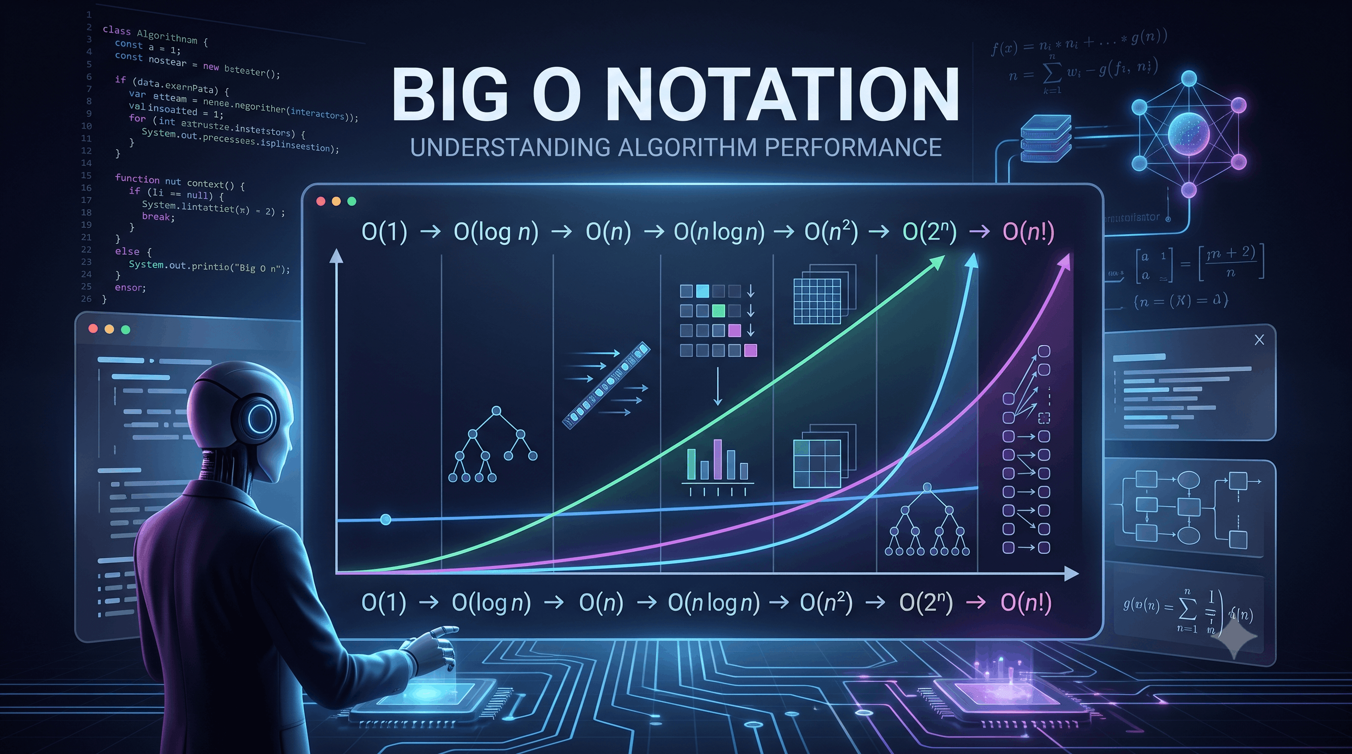
These represent different growth rates.

The Most Important Big O Complexities

For beginners, focus on these:

Let's understand them one by one.

O(1) — Constant Time

O(1) means the amount of work does not grow with the input size.

For example:

def get_first(numbers):
    return numbers[0]

Whether the array contains:

10 items

or:

10 million items

we only access one element.

Conceptually:

n = 10        → 1 operation
n = 1,000     → 1 operation
n = 1,000,000 → 1 operation

Therefore:

O(1)

Another O(1) Example

Accessing an array element by index:

numbers[500]

Assuming a standard random-access array, accessing a known index takes constant time.

The array might contain:

100 elements

or:

1 billion elements

The operation doesn't require scanning all elements.

O(log n) — Logarithmic Time

Now things get interesting.

O(log n) algorithms repeatedly reduce the problem size.

A classic example is Binary Search.

Suppose you have:

1,000,000

sorted items.

Instead of checking one at a time, binary search repeatedly cuts the search space in half.

1,000,000
     ↓
500,000
     ↓
250,000
     ↓
125,000
     ↓
62,500
     ↓
...
     ↓
1

You need surprisingly few steps.

For roughly one million elements:

log₂(1,000,000) ≈ 20

So binary search can find an element in around 20 comparisons in the idealized model.

That's why logarithmic algorithms are extremely powerful.

O(n) — Linear Time

An O(n) algorithm generally processes each input element once.

Example:

def find_sum(numbers):
    total = 0

    for number in numbers:
        total += number

    return total

If there are:

10 numbers

we process roughly 10 elements.

If there are:

1,000 numbers

we process roughly 1,000 elements.

If there are:

1,000,000 numbers

we process roughly 1,000,000 elements.

Therefore:

O(n)

Linear Search

A classic O(n) algorithm is Linear Search.

START

FOR each element

    IF element == target
        RETURN FOUND

END FOR

RETURN NOT FOUND

In the worst case, we may need to inspect every element.

Therefore:

Time Complexity = O(n)

O(n log n) — Linearithmic Time

This complexity often appears in efficient sorting algorithms.

Examples include:

• Merge Sort
• Heap Sort
• Average-case Quick Sort

The basic idea combines:

n

with:

log n

giving:

O(n log n)

For large datasets, O(n log n) is generally much more practical than O(n²).

O(n²) — Quadratic Time

This is where algorithms can start becoming problematic.

A common example is a nested loop:

for i in range(n):
    for j in range(n):
        print(i, j)

For:

n = 10

roughly:

100

iterations.

For:

n = 100

roughly:

10,000

iterations.

For:

n = 1,000

roughly:

1,000,000

iterations.

That's:

O(n²)

Visualizing Quadratic Growth

Consider:

n = 10
n² = 100

n = 100
n² = 10,000

n = 1,000
n² = 1,000,000

n = 10,000
n² = 100,000,000

The input grows by a factor of 10.

The work grows by a factor of 100.

That's why nested loops deserve attention.

Example: Comparing Every Pair

Suppose we want to compare every pair of numbers.

for i in range(len(numbers)):
    for j in range(i + 1, len(numbers)):
        compare(numbers[i], numbers[j])

There are potentially many pairs.

This is typically:

O(n²)

This pattern appears in many brute-force algorithms.

O(2ⁿ) — Exponential Time

Exponential complexity becomes dangerous very quickly.

A simple example is generating all subsets of a set.

For n elements, the number of subsets is:

2ⁿ

Consider:

n = 5
→ 32

n = 10
→ 1,024

n = 20
→ 1,048,576

n = 30
→ 1,073,741,824

The growth is explosive.

Algorithms with exponential complexity are often practical only for relatively small inputs unless special optimizations or problem-specific techniques are available.

O(n!) — Factorial Time

Factorial growth is even more extreme.

n! = n × (n-1) × (n-2) × ... × 1

For example:

5! = 120

But:

10! = 3,628,800

and:

20! = 2,432,902,008,176,640,000

Factorial complexity appears in brute-force approaches to problems involving permutations.

It becomes impractical extremely quickly.

Big O Growth Comparison

A useful mental model is:

Best
 │
 │ O(1)
 │
 │ O(log n)
 │
 │ O(n)
 │
 │ O(n log n)
 │
 │ O(n²)
 │
 │ O(2ⁿ)
 │
 │ O(n!)
 │
Worst

As you move downward, the growth rate generally becomes more problematic.

Important: Big O Is About Growth

Suppose Algorithm A takes:

5n

operations.

Algorithm B takes:

100n

operations.

Both are:

O(n)

because both grow linearly with n.

Big O focuses primarily on the growth rate, not exact execution time.

Why Do We Ignore Constants?

Suppose:

T(n) = 5n + 20

For Big O analysis, we simplify this to:

O(n)

Why?

Because as n becomes extremely large, the dominant growth term matters most.

For example:

5n + 20

is fundamentally linear.

Another Example

Consider:

T(n) = 3n² + 10n + 50

The dominant term is:

n²

Therefore:

O(n²)

We don't usually care about the constants and lower-order terms when expressing asymptotic complexity.

How to Analyze a Simple Algorithm

Consider:

x = numbers[0]
print(x)

There is no loop over the input.

Therefore:

O(1)

Now:

for number in numbers:
    print(number)

We process every element.

Therefore:

O(n)

Now:

for i in numbers:
    for j in numbers:
        print(i, j)

Two nested loops each depend on n.

Therefore:

O(n²)

Sequential Loops

Consider:

for x in numbers:
    print(x)

for x in numbers:
    print(x)

Some beginners think this is:

O(n²)

But it isn't.

The loops run sequentially:

n + n

which is:

2n

Drop the constant:

O(n)

So:

Sequential loops usually add their complexities.

Nested Loops

Now consider:

for x in numbers:
    for y in numbers:
        print(x, y)

The inner loop executes n times for every outer iteration.

Therefore:

n × n = n²

So:

O(n²)

This distinction is extremely important.

Different-Sized Loops

Consider:

for i in range(n):
    print(i)

for j in range(m):
    print(j)

Complexity:

O(n + m)

If nested:

for i in range(n):
    for j in range(m):
        print(i, j)

Complexity:

O(n × m)

So always consider what each loop depends on.

If Statements

An if statement by itself doesn't automatically make an algorithm complex.

Example:

if x > 10:
    print("Large")
else:
    print("Small")

This is:

O(1)

assuming the condition itself is constant-time.

The important thing is what happens inside the branches.

Complexity of a Function

Consider:

def process(numbers):

    total = 0

    for number in numbers:
        total += number

    return total

The loop runs n times.

Therefore:

Time Complexity = O(n)

Space Complexity

So far we've talked about time complexity.

But algorithms also consume memory.

This brings us to:

Space Complexity

Space complexity describes how much additional memory an algorithm requires as input size grows.

For example:

def sum_numbers(numbers):
    total = 0

    for number in numbers:
        total += number

    return total

We only create a few additional variables.

Therefore, the auxiliary space is:

O(1)

even though the input itself contains n elements.

Example of O(n) Space

Consider:

def copy_numbers(numbers):
    result = []

    for number in numbers:
        result.append(number)

    return result

We create another collection containing n elements.

Therefore:

Auxiliary Space = O(n)

This introduces an important trade-off:

Sometimes we use more memory to make an algorithm faster.

Time vs Space

Algorithm design often involves balancing:

Speed
   ↕
Memory

For example:

Algorithm A
Time:  O(n)
Space: O(1)

versus:

Algorithm B
Time:  O(n)
Space: O(n)

Both may have the same time complexity but very different memory requirements.

Later in this series, we'll study these trade-offs in depth.

Best Case, Average Case and Worst Case

Big O is often discussed in terms of the worst case, but algorithms can have different performance depending on the input.

Consider Linear Search:

[10, 20, 30, 40, 50]

Searching for 10:

First element

Best case:

O(1)

Searching for 50:

Check all elements

Worst case:

O(n)

If the target is somewhere in the middle, the average behavior is different again.

Why Worst Case Matters

Worst-case analysis gives us a useful guarantee.

If an algorithm is:

O(n)

we know that its work won't grow faster than the stated asymptotic bound under the relevant assumptions.

This makes complexity analysis useful when designing systems that need predictable behavior.

Big O Is Not Actual Seconds

This is a common misconception.

Suppose:

Algorithm A = O(n)
Algorithm B = O(n²)

It doesn't necessarily mean Algorithm A is always faster for every input.

A highly optimized O(n²) algorithm might beat a poorly implemented O(n) algorithm for very small datasets.

Big O tells us about scalability, not a universal stopwatch result.

A Real-World Example: Searching Users

Imagine a website has:

1,000 users

A linear search might be perfectly fine.

But now imagine:

100 million users

Scanning every user for every request could become expensive.

You may instead use:

• Hash tables
• Database indexes
• Binary search
• Caching
• Search indexes
• Specialized data structures

This is where algorithm knowledge becomes practical software engineering.

Why Databases Use Indexes

Suppose you have a database table containing millions of users.

Without an appropriate index, finding a specific record may require scanning many rows.

An index can dramatically reduce the amount of work needed to locate data.

The underlying idea is closely connected to algorithmic efficiency:

Don't examine information you don't need to examine.

This principle appears everywhere in computer science.

The Most Important Comparison

Consider:

O(n)

versus:

O(log n)

For:

n = 1,000,000

A linear algorithm may need roughly:

1,000,000

units of work in the worst case.

A logarithmic algorithm might need around:

20

halving steps.

That's an enormous difference.

Why Algorithm Choice Matters

Suppose you have two approaches:

Approach A

O(n²)

Approach B

O(n log n)

For small data:

10 elements

the difference may be insignificant.

But with:

1,000,000 elements

the difference becomes dramatic.

This is why learning algorithms isn't about solving toy programming problems.

It teaches you how to build systems that scale.

Big O Cheat Sheet

Keep this table handy:

How to Improve Algorithm Complexity

Suppose you have an O(n²) solution.

Don't immediately start optimizing random lines of code.

Ask:

Can I avoid repeated work?

Maybe you are calculating the same result repeatedly.

Can I use a better data structure?

A hash table might replace repeated searching.

Can I divide the problem?

Binary search is a classic example.

Can I sort once and then search efficiently?

Sorting can enable faster subsequent operations.

Can I trade memory for speed?

Caching and lookup tables are common examples.

Algorithm optimization is often about changing the strategy, not merely making the code shorter.

A Practical Example

Suppose we want to determine whether an array contains duplicates.

A brute-force approach might compare every pair:

for i in range(n):
    for j in range(i + 1, n):
        if numbers[i] == numbers[j]:
            return True

Worst-case complexity:

O(n²)

But we could use a set:

seen = set()

for number in numbers:

    if number in seen:
        return True

    seen.add(number)

return False

This can achieve approximately:

O(n)

average-case time with:

O(n)

additional space.

We've traded memory for speed.

That's algorithm design.

A Critical Lesson

Never optimize based only on how complicated code looks.

This:

for x in data:
    ...

may be perfectly efficient.

And this:

result = some_function(data)

could potentially hide an expensive operation.

What matters is the underlying algorithm and operations, not simply the number of lines of code.

The Algorithmic Mindset

When you see a programming problem, start asking:

How much data do I have?

How many times am I processing it?

Am I repeating work?

Can I eliminate possibilities?

Can I divide the problem?

Can I use a better data structure?

What happens when n becomes 1,000,000?

What happens when n becomes 1,000,000,000?

That is the beginning of serious algorithmic thinking.

Practice Problems

Before moving forward, try analyzing these yourself.

Problem 1

print(numbers[0])

What is the time complexity?

Answer:

O(1)

Problem 2

for number in numbers:
    print(number)

Answer:

O(n)

Problem 3

for i in numbers:
    for j in numbers:
        print(i, j)

Answer:

O(n²)

Problem 4

for i in range(n):
    print(i)

for j in range(n):
    print(j)

Answer:

O(n)

because:

O(n) + O(n)
= O(2n)
= O(n)

Final Takeaways

Big O notation gives us a language for talking about algorithm efficiency.

The most important complexities to remember are:

O(1)
O(log n)
O(n)
O(n log n)
O(n²)
O(2ⁿ)
O(n!)

And remember this general hierarchy:

O(1)
  ↓
O(log n)
  ↓
O(n)
  ↓
O(n log n)
  ↓
O(n²)
  ↓
O(2ⁿ)
  ↓
O(n!)

The lower-growth algorithms generally scale better.

But don't blindly assume:

"Lower Big O always means faster."

Real performance also depends on constants, implementation, hardware, memory access, data distribution, and input size.

The bigger lesson is:

An algorithm should not only solve the problem—it should solve it efficiently enough for the scale you care about.