Backpropagation Explained: How Neural Networks Learn From Their Mistakes

A neural network can contain thousands, millions, or even billions of parameters.

But here's the fascinating question:

How does it know which parameters should change when its prediction is wrong?

Imagine a neural network predicting:

Actual:     Cat
Prediction: Dog

The network knows it made a mistake because its loss function produces an error.

But that's only the beginning.

The network now needs to determine:

• Which weights contributed to the error?
• How much did each weight contribute?
• Should each weight increase or decrease?
• By how much?

This is where backpropagation comes in.

Backpropagation is one of the foundational ideas behind modern neural-network training.

At its core, it efficiently calculates gradients of the loss with respect to the network's parameters using the chain rule of calculus.

The optimizer then uses those gradients to update the parameters.

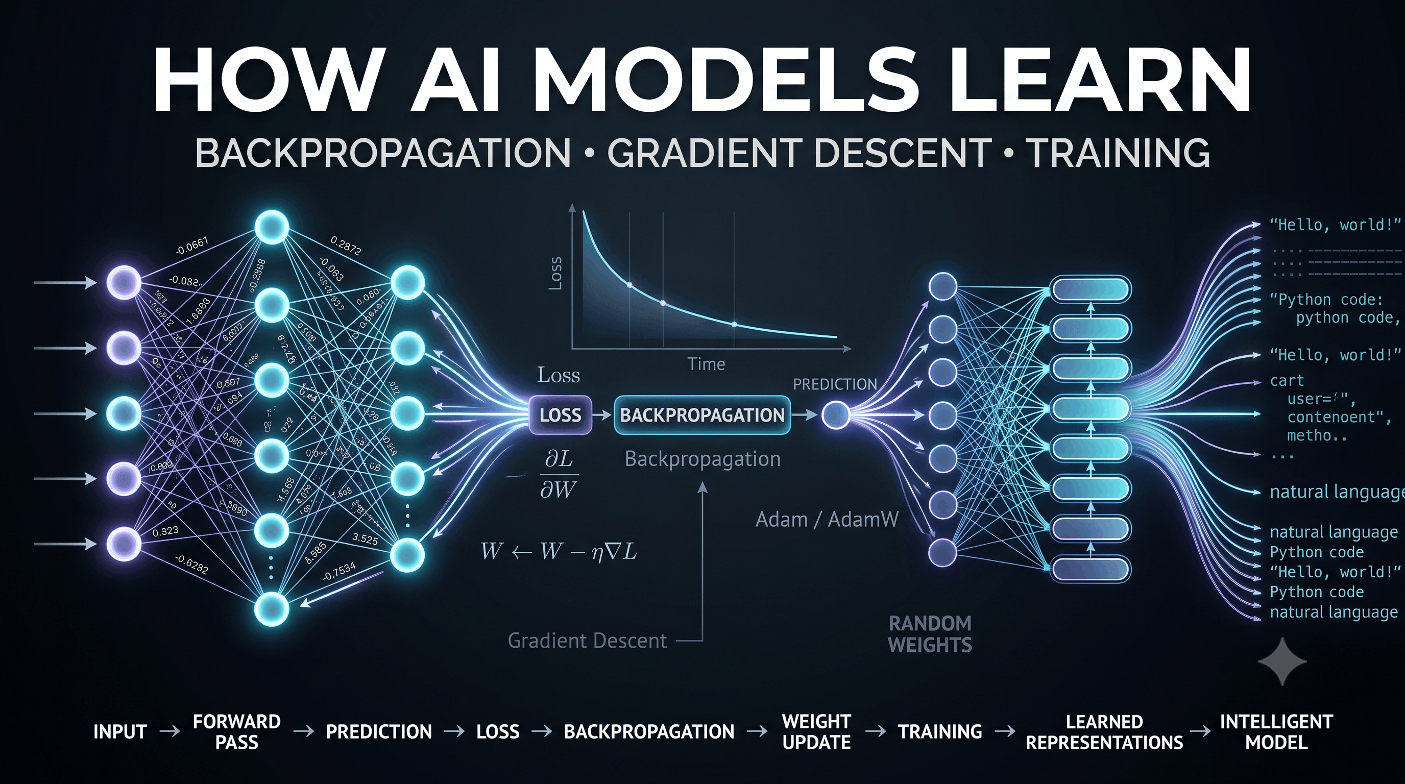
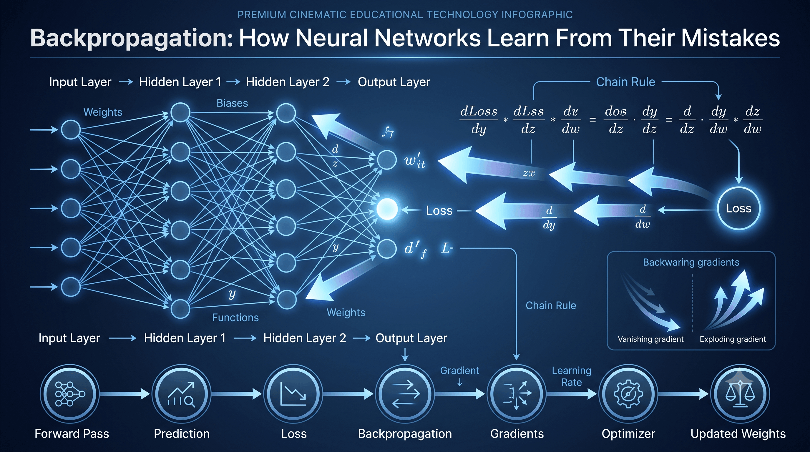
The complete process looks like:

Input
  ↓
Forward Pass
  ↓
Prediction
  ↓
Loss
  ↓
Backpropagation
  ↓
Gradients
  ↓
Optimizer
  ↓
Updated Weights
  ↓
Repeat

Let's understand every part.

Table of Contents

1. What Is Backpropagation?
2. Why Do Neural Networks Need Backpropagation?
3. The Neural Network Learning Process
4. Forward Propagation
5. Calculating the Loss
6. What Is a Gradient?
7. The Chain Rule
8. A Simple Mathematical Example
9. Backpropagation Through One Neuron
10. Backpropagation Through Multiple Layers
11. Weight Gradients
12. Bias Gradients
13. Updating Parameters
14. Backpropagation vs Gradient Descent
15. Computational Graphs
16. Automatic Differentiation
17. Vanishing Gradients
18. Exploding Gradients
19. How Modern Neural Networks Improve Training
20. Common Beginner Mistakes
21. Frequently Asked Questions
22. Key Takeaways
23. Conclusion

What Is Backpropagation?

Backpropagation is an algorithm for efficiently computing the gradients of a neural network's loss with respect to its parameters.

The name comes from the fact that information about the error is propagated backward through the network.

A simplified view:

Forward:

Input
 ↓
Layer 1
 ↓
Layer 2
 ↓
Output
 ↓
Loss


Backward:

Loss
 ↓
Layer 2 gradients
 ↓
Layer 1 gradients
 ↓
Parameter gradients

The backward pass tells us how the parameters influenced the loss.

Why Do Neural Networks Need Backpropagation?

Consider a neural network with:

1,000,000 parameters

Suppose you want to know:

How would the loss change if every parameter changed slightly?

Doing this independently for every parameter would be extremely inefficient.

Backpropagation uses the structure of the computation and the chain rule to calculate all these derivatives efficiently.

This is one reason neural networks can be trained at large scale.

The Neural Network Learning Process

A simplified training process is:

       Training Data
             ↓
       Input Features
             ↓
       Neural Network
             ↓
        Prediction
             ↓
        Loss Function
             ↓
       Backpropagation
             ↓
         Gradients
             ↓
          Optimizer
             ↓
      Updated Parameters
             ↓
           Repeat

Each training iteration gradually modifies the model parameters.

Step 1: Forward Propagation

The first stage is the forward pass.

Data moves from the input layer toward the output.

For example:

Input
 ↓
Hidden Layer 1
 ↓
Hidden Layer 2
 ↓
Output

Each neuron performs calculations using its inputs, weights, bias, and activation function.

A Single Neuron

A simplified neuron calculates:

z = wx + b

where:

• x = input
• w = weight
• b = bias
• z = weighted sum

Then an activation function may be applied:

a = f(z)

So the neuron becomes:

Input
  ↓
Weighted Sum
  ↓
Activation
  ↓
Output

Multiple Inputs

A neuron can receive many inputs.

For example:

x₁ ──w₁──┐
x₂ ──w₂──┤
x₃ ──w₃──┤→ Σ → Activation → Output
x₄ ──w₄──┘

Mathematically:

z = w₁x₁ + w₂x₂ + w₃x₃ + w₄x₄ + b

Then:

a = f(z)

This process happens across the network.

Step 2: Generate a Prediction

Suppose we're training an image classifier.

The network receives an image.

It produces:

Cat: 0.20
Dog: 0.75
Horse: 0.05

Suppose the actual label is:

Cat

The prediction is poor.

Now the network needs to determine how its parameters should change.

Step 3: Calculate the Loss

A loss function measures how wrong the prediction is.

For classification, one common choice is cross-entropy loss.

The exact formula depends on the classification setup, but conceptually:

Correct prediction
      ↓
Lower loss

Wrong prediction
      ↓
Higher loss

The network now has a numerical signal describing its error.

Step 4: Backpropagation

Now the interesting part begins.

The network asks:

How does the loss change when each parameter changes?

This is a derivative.

For a parameter w:

∂L / ∂w

This tells us how sensitive the loss L is to the parameter w.

If the value is positive, increasing the parameter would locally increase the loss.

If it is negative, increasing the parameter would locally decrease the loss.

What Is a Gradient?

A neural network usually contains many parameters.

So instead of calculating just one derivative, we calculate many.

Together, these derivatives form a gradient.

For parameters:

w₁, w₂, w₃, ..., wₙ

the gradient can be represented as:

∇L =
[
 ∂L/∂w₁,
 ∂L/∂w₂,
 ∂L/∂w₃,
 ...
 ∂L/∂wₙ
]

The gradient tells the optimizer how the loss changes with respect to the parameters.

The Chain Rule

This is the mathematical heart of backpropagation.

The chain rule tells us how to differentiate a composition of functions.

Consider:

x
 ↓
f
 ↓
g
 ↓
L

So:

L = g(f(x))

The derivative is:

dL/dx =
(dL/dg)
×
(dg/df)
×
(df/dx)

The derivatives are multiplied along the path.

This allows us to work backward through a sequence of calculations.

A Simple Example of the Chain Rule

Suppose:

y = 2x

and:

L = y²

If:

x = 3

then:

y = 6

and:

L = 36

Now we want:

dL/dx

Using the chain rule:

dL/dx =
dL/dy × dy/dx

We know:

dL/dy = 2y

and:

dy/dx = 2

Therefore:

dL/dx = 2y × 2

At y = 6:

dL/dx = 24

Backpropagation applies this same idea to much larger computational graphs.

Backpropagation Through One Neuron

Let's consider a very simple neuron.

x
 ↓
w
 ↓
z = wx + b
 ↓
a = f(z)
 ↓
Loss

We want:

∂L/∂w

The loss depends on w through several intermediate calculations.

Using the chain rule:

∂L/∂w
=
∂L/∂a
×
∂a/∂z
×
∂z/∂w

This is the key idea.

Rather than calculating the entire derivative from scratch, we multiply local derivatives.

Why This Is Powerful

Imagine a network with many layers:

x
 ↓
Layer 1
 ↓
Layer 2
 ↓
Layer 3
 ↓
Layer 4
 ↓
Loss

The chain rule allows us to calculate gradients by moving backward:

Loss
 ↓
Layer 4
 ↓
Layer 3
 ↓
Layer 2
 ↓
Layer 1

Each layer passes gradient information to the previous layer.

Backpropagation Through Multiple Layers

Consider:

Input
 ↓
Hidden Layer 1
 ↓
Hidden Layer 2
 ↓
Output
 ↓
Loss

During the backward pass:

Loss
 ↓
Output gradient
 ↓
Hidden Layer 2 gradient
 ↓
Hidden Layer 1 gradient
 ↓
Input-side gradients

Each layer receives information about how its outputs affected the loss.

It can then calculate gradients for its own parameters.

Weight Gradients

For a weight w, we calculate:

∂L/∂w

This answers:

If I change this weight slightly, how will the loss change?

The optimizer can then use this information.

For basic Gradient Descent:

w_new =
w_old -
η × ∂L/∂w

where η is the learning rate.

Bias Gradients

Biases also have gradients.

For a bias b:

∂L/∂b

The update is similarly:

b_new =
b_old -
η × ∂L/∂b

Every trainable parameter can receive its own gradient.

Putting It Together

The complete process becomes:

Forward Pass
     ↓
Prediction
     ↓
Loss
     ↓
Backward Pass
     ↓
Gradients
     ↓
Optimizer
     ↓
Update Weights + Biases
     ↓
Next Training Step

This happens repeatedly.

Backpropagation vs Gradient Descent

These terms are often confused.

They are not the same thing.

Backpropagation

Calculates gradients.

Gradient Descent

Uses gradients to update parameters.

Think of it like this:

Backpropagation
      ↓
"What direction should each parameter move?"
      ↓
Gradient

Optimizer
      ↓
"How should we actually update it?"
      ↓
New Parameters

Backpropagation vs Optimizer

Modern training is better described as:

Forward Pass
     ↓
Loss
     ↓
Backpropagation
     ↓
Gradient
     ↓
Optimizer
     ↓
Parameter Update

The optimizer could be:

• SGD
• SGD + Momentum
• Adam
• AdamW
• RMSProp

Backpropagation supplies the gradients.

The optimizer determines how to use them.

Computational Graphs

A computational graph represents calculations as connected operations.

For example:

x ──→ Multiply ──→ Add ──→ Activation ──→ Loss
        ↑            ↑
        w            b

During the forward pass:

Left → Right

During backpropagation:

Right → Left

The backward pass calculates derivatives for the operations encountered along the way.

Local Gradients

Each operation can calculate a local derivative.

For example:

z = x + y

Then:

∂z/∂x = 1
∂z/∂y = 1

For:

z = xy

we have:

∂z/∂x = y
∂z/∂y = x

Backpropagation combines these local derivatives using the chain rule.

Automatic Differentiation

Modern Deep Learning frameworks generally don't require developers to manually calculate every derivative.

Frameworks such as:

• PyTorch
• TensorFlow
• JAX

provide automatic differentiation mechanisms.

You define mathematical operations.

The framework tracks the computation.

Then it can calculate gradients automatically.

Conceptually:

Define Model
     ↓
Forward Pass
     ↓
Loss
     ↓
Automatic Differentiation
     ↓
Gradients

This is one reason modern neural-network development is practical.

A Tiny PyTorch Example

A conceptual example:

import torch

x = torch.tensor(3.0, requires_grad=True)

y = x ** 2

y.backward()

print(x.grad)

The derivative of:

y = x²

is:

dy/dx = 2x

At:

x = 3

the gradient is:

6

The framework calculates it automatically.

What Happens During .backward()?

In frameworks such as PyTorch, a backward operation triggers gradient computation through the tracked computation graph.

Conceptually:

y
 ↓
Backward
 ↓
Calculate dy/dx
 ↓
Store gradient

This is an implementation of automatic differentiation using reverse-mode differentiation for the relevant computation.

Why Reverse-Mode Differentiation?

Neural networks often have:

Many parameters
+
One scalar loss

For example:

10,000,000 parameters
        ↓
     1 loss

Reverse-mode automatic differentiation is particularly efficient for this structure because it can calculate gradients of the scalar loss with respect to many parameters in one backward pass.

This is closely related to the way backpropagation works.

Vanishing Gradients

Backpropagation introduces an important challenge.

Remember:

Chain Rule
=
Multiplication of derivatives

Suppose many derivatives are smaller than 1.

For example:

0.5 × 0.5 × 0.5 × 0.5 × 0.5

The result becomes very small.

In a deep network, repeated multiplication can cause gradients to shrink dramatically.

This is called the:

Vanishing Gradient Problem

Why Vanishing Gradients Are a Problem

Suppose:

Layer 10 → Gradient = 0.8
Layer 9  → 0.4
Layer 8  → 0.2
Layer 7  → 0.05
Layer 6  → 0.01

Earlier layers may receive extremely small gradients.

Their parameters barely change.

As a result, learning can become very slow.

Exploding Gradients

The opposite problem can occur.

Suppose derivatives repeatedly multiply by values greater than 1:

2 × 2 × 2 × 2 × 2

The result grows quickly.

This can create:

Very Large Gradients
        ↓
Huge Parameter Updates
        ↓
Unstable Training

This is known as the:

Exploding Gradient Problem

How Do We Reduce These Problems?

Modern neural networks use several techniques.

Better initialization

Weights can be initialized using methods designed to keep activations and gradients in reasonable ranges.

Examples include:

• Xavier/Glorot initialization
• He initialization

Appropriate activation functions

Some activation functions can work better than others in deep networks.

ReLU and its variants became extremely important partly because they help avoid some of the gradient-saturation behavior associated with older activation functions.

Normalization

Techniques such as:

• Batch Normalization
• Layer Normalization

can improve training behavior in appropriate architectures.

Residual Connections

Residual networks introduce shortcut connections:

Input ───────────────→ +
  ↓                    ↑
Layer 1 → Layer 2 ────┘

Instead of forcing every layer to learn an entirely new representation, the architecture allows information and gradients to flow through shortcut paths.

This became a major idea in deep neural networks.

Gradient Clipping

When gradients become excessively large, clipping can limit their magnitude.

Backpropagation and Activation Functions

Activation functions affect gradients.

Common functions include:

• ReLU
• Sigmoid
• Tanh
• GELU
• Softmax

For example, the ReLU function is:

f(x) = max(0, x)

Its derivative is approximately:

0, x < 0
1, x > 0

This simple behavior helped make ReLU-based networks easier to optimize than many older architectures.

Backpropagation Does Not "Understand" the Network

This is an important conceptual point.

Backpropagation doesn't understand:

• Cats
• Dogs
• Language
• Images
• Meaning

It performs mathematical differentiation.

The network learns useful representations because the optimization process repeatedly adjusts parameters based on the training objective.

How a Neural Network Learns "Cat"

Suppose an image contains a cat.

Initially:

Cat Probability = 0.12

The loss is high.

Backpropagation calculates gradients.

The optimizer updates parameters.

Next time:

Cat Probability = 0.25

Then:

0.48

Then:

0.76

Then:

0.94

After many examples and updates, the network can learn internal representations that help it distinguish cats from other objects.

Backpropagation Across a Deep Network

Imagine:

Pixels
  ↓
Edges
  ↓
Shapes
  ↓
Textures
  ↓
Object Parts
  ↓
Objects
  ↓
Prediction

This is a conceptual simplification, but it illustrates hierarchical representation learning.

The forward pass produces the prediction.

The backward pass provides gradient information that helps adjust the parameters responsible for these representations.

The Complete Neural Network Training Cycle

Let's put everything together:

              Training Data
                    ↓
              Input Features
                    ↓
             ┌──────────────┐
             │ Neural       │
             │ Network      │
             └──────────────┘
                    ↓
               Forward Pass
                    ↓
                Prediction
                    ↓
               Loss Function
                    ↓
             Backpropagation
                    ↓
                 Gradients
                    ↓
                Optimizer
                    ↓
             Updated Weights
                    ↓
               Next Batch
                    ↓
                 Repeat

After many iterations:

Better Parameters
       ↓
Better Predictions
       ↓
Lower Loss

At least on the training objective—and ideally on unseen data as well.

Backpropagation in Modern AI

Backpropagation isn't limited to simple neural networks.

It is foundational to training many modern Deep Learning architectures, including systems based on:

• Convolutional neural networks
• Transformers
• Large language models
• Vision models
• Speech models
• Multimodal models

The architectures may be dramatically more sophisticated, but gradient-based optimization remains central to training many of them.

What About Large Language Models?

Large Language Models contain enormous numbers of parameters.

A simplified training process looks like:

Text
 ↓
Tokens
 ↓
Transformer
 ↓
Predicted Tokens
 ↓
Loss
 ↓
Backpropagation
 ↓
Gradients
 ↓
Optimizer
 ↓
Updated Parameters

This process is repeated across enormous amounts of training data.

The mathematics is conceptually the same, even though the scale is vastly larger.

Common Beginner Mistakes

Mistake 1: Thinking Backpropagation Means "Sending the Answer Back"

Backpropagation doesn't send the correct answer backward.

It propagates gradient information backward through the computational graph.

Mistake 2: Thinking Backpropagation Updates Weights

Strictly speaking:

Backpropagation computes gradients.

The optimizer uses those gradients to update parameters.

Mistake 3: Confusing Loss With Gradient

Loss:

How wrong is the prediction?

Gradient:

How does the loss change if the parameters change?

Mistake 4: Thinking Bigger Networks Automatically Learn Better

More parameters can increase model capacity, but larger models also introduce:

• Greater computational cost
• Greater memory requirements
• More complex optimization
• Potential generalization challenges

Architecture, data, optimization, and regularization all matter.

Frequently Asked Questions

What is backpropagation in simple words?

Backpropagation is a method for calculating how much each parameter in a neural network contributed to the model's error.

Is backpropagation an optimization algorithm?

Not exactly. Backpropagation calculates gradients. An optimizer such as SGD or Adam uses those gradients to update the parameters.

What mathematical concept makes backpropagation possible?

The chain rule of calculus.

What is a gradient?

A gradient contains derivatives describing how the loss changes with respect to the model's parameters.

What is the difference between forward propagation and backpropagation?

Forward propagation calculates the model's prediction. Backpropagation works backward from the loss to calculate gradients.

Does backpropagation happen during inference?

Normally, no. During inference, you typically only perform the forward pass. Gradient computation is generally unnecessary unless you're doing a specialized procedure.

Why are vanishing gradients a problem?

Very small gradients can cause early layers to learn extremely slowly.

Why do gradients explode?

Repeated multiplication during backpropagation can sometimes produce extremely large gradients.

What is automatic differentiation?

Automatic differentiation is a computational technique that systematically calculates derivatives of programs composed of differentiable operations.

Is backpropagation used to train ChatGPT-like models?

Gradient-based backpropagation is fundamental to training modern neural networks, including Transformer-based language models.

Key Takeaways

• Backpropagation calculates gradients of the loss with respect to neural-network parameters.
• It works backward through the computational graph.
• The chain rule is the mathematical foundation.
• The forward pass produces predictions.
• The loss function measures error.
• Backpropagation calculates gradients.
• An optimizer uses those gradients to update parameters.
• Backpropagation itself isn't the same as Gradient Descent.
• Automatic differentiation allows modern frameworks to calculate gradients automatically.
• Very deep networks can experience vanishing or exploding gradients.
• Initialization, normalization, activation functions, residual connections, and gradient clipping can help training.
• Backpropagation is fundamental to training many modern Deep Learning architectures.

Conclusion

Backpropagation is one of those ideas that looks intimidating when you first encounter the mathematics.

But the fundamental idea is beautifully simple:

Make a prediction → measure the error → trace that error backward → calculate how each parameter should change → update the parameters.

The magic of modern Deep Learning doesn't come from a neural network simply making predictions.

It comes from repeating this process over and over again across enormous amounts of data.

The network gradually adjusts billions of tiny numerical parameters until useful patterns emerge.

And that brings us to another foundational question:

What exactly is a neural network made of?

We've talked about layers, neurons, weights, biases, and activation functions—but we haven't yet built one from the ground up.