How AI Models Learn: Backpropagation, Gradient Descent & Training Explained

When you ask ChatGPT a question and it produces a useful answer, it can feel almost magical.

But underneath that intelligence is something surprisingly mathematical.

The model does not start with knowledge.

It starts with numbers.

Millions, billions, or even trillions of numerical parameters are initialized, and through an enormous number of training iterations, those numbers are repeatedly adjusted.

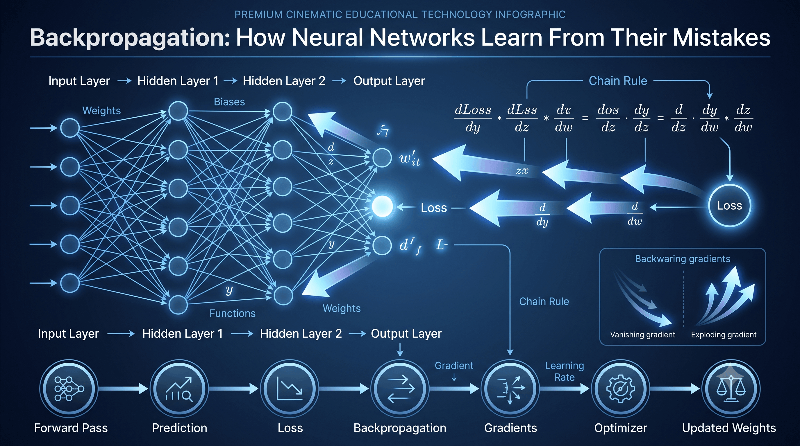
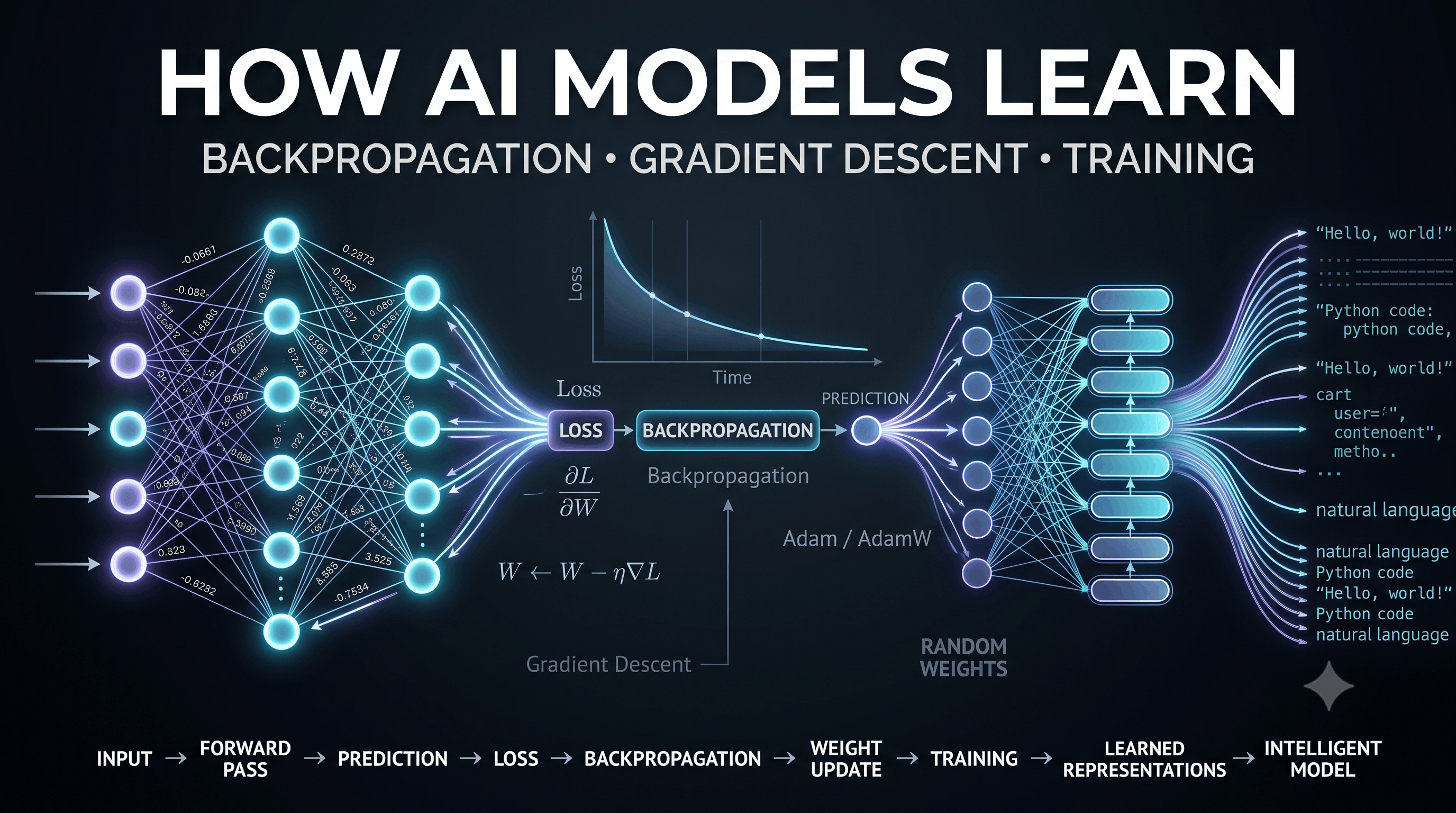
The basic process looks like this:

Input
  ↓
Model makes prediction
  ↓
Prediction is compared with correct answer
  ↓
Loss is calculated
  ↓
Gradients are calculated
  ↓
Backpropagation determines how parameters contributed to the error
  ↓
Optimizer updates parameters
  ↓
Model becomes slightly better
  ↓
Repeat billions/trillions of times

This is the fundamental idea behind modern deep learning.

So how does a collection of random numbers eventually become a neural network capable of recognizing images, translating languages, writing code, or generating text?

Let's build the entire process from first principles.

Table of Contents

1. What Does It Mean for AI to Learn?
2. Parameters: The Numbers Inside a Model
3. Weights and Biases
4. The Forward Pass
5. From Prediction to Loss
6. What Is a Loss Function?
7. Cross-Entropy Loss
8. What Is a Gradient?
9. The Intuition Behind Gradient Descent
10. Backpropagation
11. The Chain Rule
12. Updating Model Parameters
13. Learning Rate
14. Batch, Mini-Batch, and Epoch
15. Stochastic Gradient Descent
16. Momentum
17. Adam and AdamW
18. The Complete Training Loop
19. A Tiny Numerical Example
20. How Neural Networks Learn Features
21. Why Training Deep Networks Is Difficult
22. Vanishing and Exploding Gradients
23. Weight Initialization
24. Normalization
25. Overfitting and Underfitting
26. Training vs Validation
27. How Transformers Learn
28. How LLMs Learn Language
29. Pretraining
30. Fine-Tuning
31. Instruction Tuning
32. The Role of GPUs
33. Mixed Precision and Distributed Training
34. Checkpoints
35. Training vs Inference
36. Common Misconceptions
37. Frequently Asked Questions
38. Key Takeaways
39. Conclusion

1. What Does It Mean for AI to Learn?

Let's begin with the most important question.

What does "learning" actually mean?

For humans, learning might mean:

Seeing something repeatedly and developing an understanding of it.

For a neural network, learning means something much more precise:

Adjusting its parameters so that its predictions become better according to a defined objective.

Suppose we want a model to predict whether an image contains a cat.

We provide:

Image → Model → Prediction

Initially, the model might say:

Cat: 31%
Dog: 69%

But the correct answer is:

Cat: 100%

The model made an error.

Training gives the model a mechanism to answer:

"How should I change my internal parameters so that my next prediction is better?"

That mechanism is built around:

Loss
Gradients
Backpropagation
Optimization

2. Parameters: The Numbers Inside a Model

A neural network contains parameters.

The most important parameters are:

• weights
• biases

A simple neural network might have thousands of parameters.

A modern large language model may have billions or more.

Conceptually:

Model
│
├── Layer 1
│   ├── Weight matrix
│   └── Bias
│
├── Layer 2
│   ├── Weight matrix
│   └── Bias
│
├── Layer 3
│   ├── Weight matrix
│   └── Bias
│
└── Output Layer
    ├── Weight matrix
    └── Bias

These parameters are what training changes.

The architecture defines how computation works.

The parameters determine what the trained model has learned.

3. Weights and Biases

Consider a simple neuron:

x₁ ──w₁──┐
          │
x₂ ──w₂──┼──→ Σ → activation → output
          │
x₃ ──w₃──┘

The neuron calculates something like:

[
z = w_1x_1 + w_2x_2 + w_3x_3 + b
]

Where:

• (x) = input
• (w) = weight
• (b) = bias
• (z) = weighted sum

Then an activation function may transform the result.

For example:

[
y = ReLU(z)
]

The model's behavior depends heavily on the values of these parameters.

Training is largely the process of finding useful parameter values.

4. The Forward Pass

The first major step during training is the forward pass.

The input moves through the network.

For example:

Input
  ↓
Layer 1
  ↓
Activation
  ↓
Layer 2
  ↓
Activation
  ↓
Layer 3
  ↓
Prediction

Suppose the model receives:

Input: "The capital of France is"

A language model processes the input and produces scores for possible next tokens.

Perhaps:

Paris      → 8.7
London     → 3.2
Berlin     → 2.8
Madrid     → 1.9
Apple      → -1.2

These raw scores are called logits.

The model hasn't necessarily produced a final answer yet.

The logits can be converted into probabilities using softmax.

5. From Prediction to Loss

Now we need to determine:

How wrong was the model?

That's where the loss function comes in.

Imagine the correct next token is:

Paris

But the model assigned:

Paris → 20%

That's not a very good prediction.

The loss function converts the quality of the prediction into a numerical value.

For example:

Good prediction → Low loss
Bad prediction  → High loss

The training objective becomes:

[
\text{Minimize Loss}
]

This simple idea drives much of modern machine learning.

6. What Is a Loss Function?

A loss function measures the difference between:

Prediction

and

Ground Truth

Different tasks use different loss functions.

Examples:

For example, in regression:

[
MSE = \frac{1}{n}\sum_{i=1}^{n}(y_i-\hat{y_i})^2
]

Where:

• (y) = actual value
• (\hat y) = predicted value

The model tries to reduce this number.

7. Cross-Entropy Loss

Cross-entropy is especially important for classification and language models.

Suppose the correct answer has probability (p).

The loss can be expressed as:

[
L = -\log(p)
]

Consider:

Correct probability = 0.9
Loss ≈ 0.105

But:

Correct probability = 0.1
Loss ≈ 2.303

So assigning high probability to the correct answer produces a smaller loss.

This creates a useful training signal.

The model learns:

Increase probability for correct answers and decrease probability for incorrect ones.

8. What Is a Gradient?

Now we reach one of the most important concepts in AI.

A gradient tells us how the loss changes when a parameter changes.

Imagine you're standing on a mountain.

You want to reach the lowest point.

You need to know:

Which direction goes downhill?

The gradient provides that information.

For a parameter (w):

[
\frac{\partial L}{\partial w}
]

means:

How much does the loss change if we slightly change (w)?

If the gradient is positive:

Increasing w → increases loss

If the gradient is negative:

Increasing w → decreases loss

The model uses this information to decide how to modify its parameters.

9. The Intuition Behind Gradient Descent

Imagine this landscape:

Loss
 ↑
 │        *
 │      *   *
 │    *       *
 │  *           *
 │ *             *
 │        ↓
 │      Minimum
 └──────────────────→ Parameter

The goal is to reach the minimum loss.

Gradient descent says:

Move the parameters in the direction that reduces the loss.

The basic update equation is:

[
w_{new}=w_{old}-\eta\frac{\partial L}{\partial w}
]

Where:

• (w) = parameter
• (L) = loss
• (\eta) = learning rate

The minus sign is important.

We move against the gradient.

10. Backpropagation

Gradient descent tells us:

What should happen to the parameters?

But we still need to calculate:

How did every parameter contribute to the final error?

That's the job of backpropagation.

During the forward pass:

Input
 ↓
Layer 1
 ↓
Layer 2
 ↓
Output
 ↓
Loss

During backpropagation:

Loss
 ↑
Layer 2
 ↑
Layer 1
 ↑
Input

The error signal travels backward through the network.

The model calculates gradients for its parameters.

11. The Chain Rule

Backpropagation relies heavily on the mathematical chain rule.

Suppose:

[
y=f(g(x))
]

Then:

\frac{dy}{dg}
\frac{dg}{dx}
]

A neural network is essentially a large composition of functions.

For example:

x
 ↓
f₁
 ↓
f₂
 ↓
f₃
 ↓
Loss

The chain rule allows us to calculate:

[
\frac{\partial Loss}{\partial w}
]

for parameters deep inside the network.

This is why backpropagation is so powerful.

12. Updating Model Parameters

Once the gradients are calculated, the optimizer updates the parameters.

The simplest version is:

[
w \leftarrow w-\eta\nabla_w L
]

Imagine:

Current weight = 0.50
Gradient       = 0.20
Learning rate  = 0.01

Then:

[
w_{new}=0.50-(0.01)(0.20)
]

[
w_{new}=0.498
]

It's a tiny change.

And that's important.

A neural network usually doesn't suddenly become intelligent.

It improves through enormous numbers of tiny updates.

13. Learning Rate

The learning rate determines the size of each update.

Imagine you're walking downhill.

Learning rate too small

step → step → step → step → step

Training may be extremely slow.

Learning rate too large

       ↗
minimum
       ↘
       ↗

The optimizer may overshoot the minimum.

Appropriate learning rate

\        /
 \      /
  \    /
   \__/

The model gradually approaches a useful solution.

Learning rate is one of the most important hyperparameters in training.

14. Batch, Mini-Batch, and Epoch

Training usually involves huge datasets.

You don't necessarily process the entire dataset in one operation.

Instead, data is divided into batches.

Suppose we have:

1,000,000 training examples

And batch size is:

1,000

Then one complete pass through the dataset requires:

[
\frac{1,000,000}{1,000}=1,000
]

training steps.

One complete pass through the dataset is called an epoch.

Dataset
│
├── Batch 1
├── Batch 2
├── Batch 3
├── ...
└── Batch 1000

          ↓

        1 Epoch

15. Stochastic Gradient Descent

Instead of calculating gradients using the entire dataset, we can calculate them using smaller batches.

This is called mini-batch gradient descent.

A very small batch can introduce noise into the gradient.

That isn't necessarily bad.

The noise can sometimes help the optimizer explore the loss landscape.

The general process becomes:

Select batch
     ↓
Forward pass
     ↓
Calculate loss
     ↓
Backpropagation
     ↓
Calculate gradients
     ↓
Update parameters
     ↓
Next batch

16. Momentum

Basic gradient descent can sometimes behave inefficiently.

Momentum introduces a concept similar to inertia.

Instead of considering only the current gradient, the optimizer maintains information about previous updates.

Conceptually:

Gradient
   ↓
Momentum
   ↓
Smoothed direction
   ↓
Parameter update

This can help the optimizer move more efficiently through difficult loss landscapes.

17. Adam and AdamW

Modern neural networks commonly use more sophisticated optimizers.

One of the most famous is Adam.

Adam combines ideas related to:

• momentum
• adaptive learning rates

Instead of treating every parameter identically, Adam maintains statistics about gradients and adjusts updates accordingly.

Another important optimizer is AdamW.

AdamW separates weight decay from the gradient update in a way that generally makes regularization behavior cleaner than traditional L2 regularization implemented directly inside Adam.

For modern deep learning systems, AdamW is particularly common.

18. The Complete Training Loop

Now we can combine everything.

A simplified training loop looks like this:

Initialize parameters

Repeat:

    Get a batch of training data

    ↓

    Forward pass

    ↓

    Generate predictions

    ↓

    Calculate loss

    ↓

    Backpropagation

    ↓

    Calculate gradients

    ↓

    Optimizer updates parameters

    ↓

    Repeat

In pseudocode:

for batch in dataset:

    predictions = model(batch.inputs)

    loss = loss_function(
        predictions,
        batch.targets
    )

    optimizer.zero_grad()

    loss.backward()

    optimizer.step()

This tiny loop captures the core idea behind training neural networks.

Real systems are vastly more complicated, but the conceptual structure remains.

19. A Tiny Numerical Example

Let's simplify everything dramatically.

Suppose:

[
y=wx
]

We want the model to learn:

[
y=10
]

Input:

[
x=2
]

Current weight:

[
w=3
]

The model predicts:

[
\hat y=3\times2=6
]

The prediction is wrong.

Suppose we use squared error:

[
L=(y-\hat y)^2
]

Therefore:

[
L=(10-6)^2
]

[
L=16
]

Now we calculate the gradient.

Since:

[
\hat y=wx
]

and:

[
L=(y-wx)^2
]

the derivative with respect to (w) is:

-2x(y-wx)
]

Substituting:

[
-2(2)(10-6)
]

[
=-16
]

Assume:

[
\eta=0.1
]

Then:

[
w_{new}=3-(0.1)(-16)
]

[
w_{new}=4.6
]

The model's new prediction becomes:

[
4.6\times2=9.2
]

We started with:

Prediction = 6

After one update:

Prediction = 9.2

The model moved closer to the target.

That's learning.

20. How Neural Networks Learn Features

An interesting question is:

What exactly does a neural network learn?

The answer depends on the architecture and task.

Consider an image model.

Early layers might learn patterns resembling:

Edges
Corners
Textures

Middle layers can combine these into:

Shapes
Patterns
Parts of objects

Later layers may represent:

Faces
Animals
Objects
Scenes

The network builds increasingly complex representations.

For language models, the learned representations are much more abstract.

They can encode relationships involving:

words
syntax
semantics
entities
patterns
code structures
facts
relationships
context

But these aren't necessarily stored like entries in a traditional database.

They emerge from learned parameter patterns.

21. Why Training Deep Networks Is Difficult

Training a neural network sounds simple:

Predict
→ calculate loss
→ calculate gradients
→ update weights

But large neural networks introduce serious challenges.

For example:

• billions of parameters
• enormous datasets
• expensive matrix operations
• unstable gradients
• memory constraints
• optimization difficulties
• distributed computation
• overfitting
• hardware failures
• training instability

The bigger the model becomes, the more engineering matters.

22. Vanishing and Exploding Gradients

During backpropagation, gradients are propagated through many layers.

Sometimes they become extremely small.

This is called the:

Vanishing Gradient Problem

Gradient
 ↓
0.1
 ↓
0.01
 ↓
0.001
 ↓
0.0001
 ↓
...

Eventually, early layers receive almost no useful signal.

The opposite can also happen.

Gradients may become extremely large.

That's the:

Exploding Gradient Problem

1
 ↓
10
 ↓
100
 ↓
1,000
 ↓
10,000

This can make training unstable.

Modern architectures use several techniques to improve optimization, including:

• careful initialization
• normalization
• residual connections
• appropriate activation functions
• optimizer improvements
• learning-rate schedules
• gradient clipping

23. Weight Initialization

A model cannot simply initialize every weight arbitrarily without consequences.

Poor initialization can make training unstable.

Modern initialization strategies attempt to keep activations and gradients at useful scales.

Examples include:

• Xavier/Glorot initialization
• He initialization
• specialized initialization used by modern architectures

Initialization is particularly important in deep networks.

24. Normalization

Neural networks often benefit from normalization techniques.

One widely used technique in Transformers is Layer Normalization.

Normalization helps keep activations within manageable ranges and can improve optimization stability.

Modern Transformer architectures also commonly use variants such as:

• LayerNorm
• RMSNorm

Normalization is one of the many engineering improvements that helped make very deep models practical.

25. Overfitting and Underfitting

A model can fail in two opposite ways.

Underfitting

The model hasn't learned enough.

Training performance → poor
Validation performance → poor

Overfitting

The model memorizes the training data too strongly and fails to generalize.

Training performance → excellent
Validation performance → poor

The goal is:

Learn useful patterns
        ↓
Generalize to unseen data

This distinction is critical in machine learning.

26. Training vs Validation

A good training pipeline doesn't only monitor training loss.

We also evaluate the model on data it hasn't trained on.

For example:

Dataset
│
├── Training Set
│      ↓
│   Model learns
│
└── Validation Set
       ↓
   Model is evaluated

If training loss keeps decreasing while validation performance gets worse, the model may be overfitting.

This helps engineers decide:

• when to stop training
• which hyperparameters to use
• which checkpoint to select
• whether the model generalizes

27. How Transformers Learn

Now let's connect this with the Transformer architecture from the previous article.

A Transformer processes token sequences.

For example:

The cat is sitting on the

During language-model training, the model may be asked to predict:

mat

The Transformer processes the context.

The
 ↓
cat
 ↓
is
 ↓
sitting
 ↓
on
 ↓
the
 ↓
?

It produces logits for the vocabulary.

mat       → high probability
chair     → medium probability
car       → low probability
banana    → very low probability

The correct token is known from the training data.

The loss measures how well the model predicted it.

Then:

Loss
 ↓
Backpropagation
 ↓
Gradients
 ↓
Optimizer
 ↓
Updated Transformer parameters

This happens repeatedly.

28. How LLMs Learn Language

This is one of the most important ideas in modern AI.

A large language model can be trained using next-token prediction.

Consider:

Artificial intelligence is

The training target might be:

powerful

Another example:

The Earth revolves around the

Target:

Sun

Another:

function calculateSum(a, b) {

Target might be:

return

The model repeatedly sees contexts and learns to predict what comes next.

At enormous scale, this objective forces the model to learn many statistical and structural patterns in language and other data.

29. Pretraining

The initial large-scale training phase is commonly called pretraining.

The model is exposed to a huge corpus of training data.

Conceptually:

Massive Dataset
      ↓
Tokenization
      ↓
Training Batches
      ↓
Transformer
      ↓
Predictions
      ↓
Loss
      ↓
Backpropagation
      ↓
Optimizer
      ↓
Updated Parameters
      ↓
Repeat

After a huge number of optimization steps, the resulting model contains learned representations and capabilities.

But a pretrained model isn't necessarily optimized for following instructions in the way users expect.

That's where later training stages come in.

30. Fine-Tuning

Fine-tuning takes a pretrained model and continues training it on a more specialized dataset.

For example:

General pretrained model
          ↓
   Medical dataset
          ↓
Specialized model

Or:

General pretrained model
          ↓
   Coding dataset
          ↓
Coding-focused model

Fine-tuning can adapt a model to:

• specific domains
• specific tasks
• particular styles
• specialized behavior

31. Instruction Tuning

A pretrained language model learns to predict tokens.

But users want something more useful:

Follow my instruction.

Instruction tuning helps bridge that gap.

Training examples might look conceptually like:

Instruction:
Explain recursion simply.

Response:
Recursion is a technique...

The model learns patterns connecting instructions with useful responses.

Other post-training techniques can further shape model behavior, preferences, safety, reasoning behavior, and interaction style.

The important distinction is:

Pretraining
    ↓
Learn broad patterns

Post-training
    ↓
Make the model more useful for people

32. The Role of GPUs

Training modern neural networks requires enormous amounts of computation.

A huge portion of neural-network computation consists of matrix operations.

GPUs are extremely good at performing many numerical operations in parallel.

Conceptually:

CPU

Core → sequential/general workloads

versus:

GPU

Thousands of parallel computational units
│ │ │ │ │ │ │ │
│ │ │ │ │ │ │ │
│ │ │ │ │ │ │ │
└─ Parallel numerical computation

Large AI systems may use thousands of GPUs or other accelerators during training.

The challenge isn't simply:

"Can we train the model?"

It is:

"Can we train it efficiently, reliably, and economically?"

33. Mixed Precision and Distributed Training

Modern training systems use many optimization techniques.

Mixed Precision

Instead of performing every calculation at the highest numerical precision, training can use lower-precision formats where appropriate.

Benefits can include:

• lower memory usage
• faster computation
• better hardware utilization

Distributed Training

A large model may be trained across many machines.

For example:

GPU 1 ─┐
GPU 2 ─┤
GPU 3 ─┤
GPU 4 ─┤
GPU 5 ─┤
GPU 6 ─┤──→ Distributed Training
GPU 7 ─┤
GPU 8 ─┘

At very large scales, distributed training becomes a major systems-engineering challenge.

34. Checkpoints

Training can take days, weeks, or longer.

You don't want to lose everything because a machine fails.

So training systems periodically save checkpoints.

A checkpoint can contain:

Model parameters
Optimizer state
Training step
Learning-rate state
Other training metadata

For example:

checkpoint-10000
checkpoint-20000
checkpoint-30000
...

If training fails, it may be possible to resume from a recent checkpoint.

35. Training vs Inference

Training and inference are fundamentally different workloads.

Training

Input
 ↓
Forward Pass
 ↓
Loss
 ↓
Backward Pass
 ↓
Gradients
 ↓
Parameter Update

Inference

Input
 ↓
Forward Pass
 ↓
Prediction

During ordinary inference, the model's parameters are not updated.

For an LLM:

User prompt
   ↓
Transformer
   ↓
Next-token probabilities
   ↓
Selected token
   ↓
Next-token prediction
   ↓
Repeat

This is why generating a response doesn't normally "teach" the model instantly.

36. Common Misconceptions

Misconception 1: AI learns like a human

Not exactly.

Neural-network learning is numerical optimization over parameters.

Misconception 2: The model understands everything during training

A model doesn't receive a human-like explanation of every concept.

It learns statistical and representational patterns through its training objective.

Misconception 3: Backpropagation changes the model directly

Backpropagation calculates gradients.

The optimizer uses those gradients to update parameters.

The distinction matters:

Backpropagation
      ↓
Calculates gradients

Optimizer
      ↓
Uses gradients to update parameters

Misconception 4: More training always makes a model better

Not necessarily.

Too much training can cause overfitting or other problems.

Training quality depends on:

• data
• architecture
• optimization
• compute
• hyperparameters
• evaluation

Misconception 5: A large model is intelligent because it has more parameters

Parameter count matters, but it isn't the whole story.

Model quality also depends on:

• architecture
• data quality
• training objective
• optimization
• compute
• post-training
• inference methods

37. Frequently Asked Questions

What is backpropagation in simple terms?

Backpropagation calculates how much each model parameter contributed to the prediction error.

What is gradient descent?

Gradient descent is an optimization method that updates parameters in a direction that reduces loss.

What is a learning rate?

The learning rate controls how large each parameter update is.

What is an epoch?

One complete pass through the training dataset.

What is a batch?

A group of training examples processed together before an optimizer update.

Why do we need a loss function?

The loss function gives the model a numerical signal indicating how good or bad its prediction was.

What is an optimizer?

An optimizer determines how model parameters should be updated using gradients.

What is Adam?

Adam is an adaptive optimization algorithm that combines momentum-like behavior with parameter-specific adaptive learning rates.

Why are GPUs used for AI?

Neural networks involve enormous amounts of parallel numerical computation, particularly matrix operations, which GPUs handle efficiently.

Do LLMs memorize everything they see?

Models can memorize portions of their training data, especially under certain conditions, but learning is not equivalent to storing the entire dataset as a database.

Does training happen every time I ask an AI a question?

Normally, no. Inference and training are separate processes.

38. Key Takeaways

Let's compress the entire article into one mental model.

A neural network begins with parameters.

Random Parameters
       ↓
Input
       ↓
Forward Pass
       ↓
Prediction
       ↓
Loss
       ↓
Backpropagation
       ↓
Gradients
       ↓
Optimizer
       ↓
Parameter Update
       ↓
Better Model
       ↓
Repeat

The key concepts are:

Parameters

The numbers that determine the model's behavior.

Forward Pass

The model processes input and produces a prediction.

Loss

Measures how wrong the prediction is.

Gradient

Measures how the loss changes with respect to a parameter.

Backpropagation

Efficiently calculates gradients throughout the network.

Gradient Descent

Moves parameters toward lower loss.

Optimizer

Controls how parameters are updated.

Learning Rate

Controls the size of those updates.

Batch

A group of examples processed together.

Epoch

One complete pass through the training dataset.

Pretraining

Large-scale learning of broad patterns.

Fine-Tuning

Adapting a pretrained model to a particular purpose.

39. Conclusion

We've now reached one of the most important ideas in artificial intelligence.

An AI model doesn't begin intelligent.

It begins with parameters.

Through an enormous optimization process, the model repeatedly:

Predicts
   ↓
Makes mistakes
   ↓
Measures mistakes
   ↓
Calculates gradients
   ↓
Updates parameters
   ↓
Predicts again

One update may change almost nothing.

One thousand updates may still look unimpressive.

Millions or billions of updates, combined with enormous amounts of data and computation, can produce remarkably capable models.

This is the foundation:

[
\boxed{
\text{Loss}
\rightarrow
\text{Gradients}
\rightarrow
\text{Backpropagation}
\rightarrow
\text{Optimization}
\rightarrow
\text{Learning}
}
]

And this same fundamental idea scales from a tiny neural network running on your laptop to massive Transformer models trained across large GPU clusters.

But there's a fascinating question still unanswered:

If an LLM is trained by predicting the next token, how does that simple objective turn into something capable of writing essays, solving programming problems, translating languages, and holding conversations?

That's where we go next.