Neural Networks Explained: From a Single Neuron to Modern AI

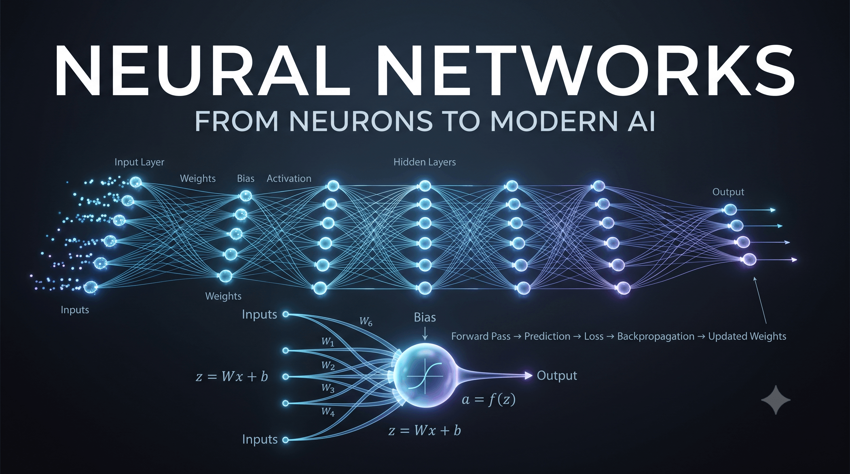
When people hear Artificial Intelligence, they often imagine something incredibly complicated.

A chatbot answering questions.

A computer recognizing faces.

An AI generating images.

A self-driving system identifying objects on a road.

A language model predicting the next word in a sentence.

Underneath many of these systems is a powerful computational idea:

The Neural Network

Neural networks are mathematical models inspired loosely by the way biological nervous systems process information.

But don't let the biological analogy confuse you.

A modern neural network is fundamentally a mathematical computation made from parameters, functions, and layers.

The basic building blocks are:

Neuron
   ↓
Weights
   ↓
Bias
   ↓
Activation Function
   ↓
Layer
   ↓
Neural Network

Once you understand these components, concepts such as Deep Learning, Transformers, Computer Vision, and Large Language Models become much easier to understand.

Let's build the idea from the ground up.

Table of Contents

1. What Is a Neural Network?
2. Why Do We Need Neural Networks?
3. The Simplest Neural Network
4. What Is an Artificial Neuron?
5. Inputs
6. Weights
7. Bias
8. Weighted Sum
9. Activation Functions
10. A Single Neuron Example
11. Multiple Neurons
12. Layers
13. Input Layer
14. Hidden Layers
15. Output Layer
16. Forward Propagation
17. Training a Neural Network
18. Loss Function
19. Backpropagation
20. Gradient Descent
21. Neural Network Example
22. Classification
23. Regression
24. Deep Neural Networks
25. Why Non-Linearity Matters
26. Common Activation Functions
27. Parameters vs Hyperparameters
28. Epochs and Batches
29. Neural Networks and Overfitting
30. Regularization
31. Modern Neural Networks
32. Neural Networks and Large Language Models
33. Common Beginner Mistakes
34. Frequently Asked Questions
35. Key Takeaways
36. Conclusion

What Is a Neural Network?

A neural network is a mathematical model composed of interconnected computational units—often called neurons—organized into layers.

A very simple neural network might look like:

Input Layer
     ↓
Hidden Layer
     ↓
Output Layer

A larger network could look like:

Input
 ↓
Layer 1
 ↓
Layer 2
 ↓
Layer 3
 ↓
Layer 4
 ↓
Output

Each layer transforms the information it receives.

Why Do We Need Neural Networks?

Traditional programming generally looks like:

Rules + Data
     ↓
Program
     ↓
Output

For example, imagine writing a program to identify spam emails.

You might manually create rules:

IF email contains "FREE MONEY"
    spam

IF email contains suspicious links
    spam

But real-world data is messy.

Spam can be written in countless ways.

Instead of manually defining every rule, Machine Learning allows a model to learn useful patterns from examples.

Training Data
     ↓
Neural Network
     ↓
Learned Parameters
     ↓
Predictions

The Simplest Neural Network

Let's start with a single neuron.

x₁ ── w₁ ──┐
            │
x₂ ── w₂ ──┤
            ├──→ Neuron → Output
x₃ ── w₃ ──┤
            │
            b

The neuron receives inputs.

Each input has an associated weight.

The neuron combines them, adds a bias, and applies an activation function.

Mathematically:

z = w₁x₁ + w₂x₂ + w₃x₃ + b

Then:

a = f(z)

where f is the activation function.

What Is an Artificial Neuron?

An artificial neuron is a mathematical function that receives inputs and produces an output.

The basic process is:

Inputs
  ↓
Multiply by weights
  ↓
Add values
  ↓
Add bias
  ↓
Activation function
  ↓
Output

A neuron isn't intelligent by itself.

Its power comes from combining huge numbers of these computations.

Inputs

Inputs represent the information given to the network.

Suppose we want to predict whether someone will purchase a product.

Our inputs might be:

x₁ = Age
x₂ = Income
x₃ = Time spent on website
x₄ = Previous purchases

These values are passed into the network.

Weights

Each input has a corresponding weight.

For example:

Age              → w₁
Income           → w₂
Website Time     → w₃
Previous Orders  → w₄

Weights determine how strongly different inputs influence the neuron's calculation.

For example:

Income → large positive weight

could mean income has a strong positive influence on the neuron's output in the learned model.

But remember:

The meaning of an individual weight depends on the architecture, data representation, and surrounding network.

The Most Important Idea

Weights are learned parameters.

The programmer doesn't normally specify the perfect values manually.

During training:

Initial Weights
      ↓
Prediction
      ↓
Loss
      ↓
Backpropagation
      ↓
Gradient
      ↓
Updated Weights

This process repeats many times.

What Is Bias?

Bias is another trainable parameter.

A simplified neuron calculates:

z = wx + b

Without the bias, the neuron has less flexibility.

Bias allows the activation function to shift.

You can think of it as an adjustable offset.

For example:

z = wx + b

Changing b changes where the activation begins responding strongly.

Weighted Sum

Let's say:

x₁ = 2
x₂ = 4

and:

w₁ = 0.5
w₂ = 0.8

with:

b = 1

Then:

z = (2 × 0.5) + (4 × 0.8) + 1

Therefore:

z = 1 + 3.2 + 1

z = 5.2

The neuron then passes 5.2 through an activation function.

Activation Functions

Why do we need an activation function?

Because without appropriate non-linear transformations, stacking multiple linear layers would still produce an overall linear transformation.

Activation functions introduce non-linearity.

Common activation functions include:

• ReLU
• Sigmoid
• Tanh
• GELU
• Softmax

ReLU

ReLU stands for:

Rectified Linear Unit

Its formula is:

f(x) = max(0, x)

So:

x = -5 → 0
x = -1 → 0
x =  0 → 0
x =  2 → 2
x =  7 → 7

ReLU became one of the most important activation functions in Deep Learning.

Sigmoid

The sigmoid function maps values approximately into the range:

0 → 1

Its mathematical form is:

σ(x) = 1 / (1 + e⁻ˣ)

For example:

Large negative → close to 0
0              → 0.5
Large positive → close to 1

Sigmoid is historically important and remains useful in specific situations, particularly when an output needs to represent a probability-like value for binary classification.

Tanh

Tanh maps values approximately into:

-1 → +1

It is defined as:

tanh(x)

It was widely used in older neural-network architectures and remains relevant in certain settings.

GELU

GELU stands for:

Gaussian Error Linear Unit

GELU is commonly used in modern Transformer architectures.

It provides a smooth non-linear transformation and has become an important activation function in modern Deep Learning.

Softmax

Softmax is commonly used to convert a vector of logits into values that sum to 1.

For example:

Cat    → 0.70
Dog    → 0.20
Horse  → 0.10

The values can be interpreted as a probability distribution over classes under the model's classification setup.

One Neuron in Action

Suppose we have:

x = 3
w = 2
b = 1

Then:

z = wx + b

Therefore:

z = (2 × 3) + 1

z = 7

If we use ReLU:

ReLU(7) = 7

The neuron outputs:

7

Multiple Neurons

One neuron isn't enough for most interesting tasks.

So we create multiple neurons.

          ┌→ Neuron 1 →┐
Input ────┼→ Neuron 2 →┼→ Next Layer
          ├→ Neuron 3 →┤
          └→ Neuron 4 →┘

Each neuron can have its own:

• Weights
• Bias
• Activation

This allows different neurons to learn different transformations.

What Is a Layer?

A layer is a collection of neurons operating together.

For example:

Input
 ↓
[Neuron 1]
[Neuron 2]
[Neuron 3]
[Neuron 4]
 ↓
Next Layer

A neural network typically contains:

Input Layer
      ↓
Hidden Layers
      ↓
Output Layer

Input Layer

The input layer receives the features.

For an image:

Pixel 1
Pixel 2
Pixel 3
...
Pixel N

For a text model, the raw text is first transformed into tokens and then into numerical representations before being processed by the network.

For a house-price model:

Area
Bedrooms
Location Features
Age
...

Hidden Layers

Layers between the input and output are called hidden layers.

For example:

Input
 ↓
Hidden Layer 1
 ↓
Hidden Layer 2
 ↓
Hidden Layer 3
 ↓
Output

The word "hidden" simply means these internal representations aren't directly the input or final output.

Output Layer

The output layer produces the model's final output.

For binary classification:

Probability = 0.87

For multi-class classification:

Cat    = 0.80
Dog    = 0.15
Horse  = 0.05

For regression:

Predicted House Price = ₹72 lakh

The output structure depends on the task.

Forward Propagation

When information travels from the input toward the output, this is called forward propagation or the forward pass.

Input
 ↓
Layer 1
 ↓
Layer 2
 ↓
Layer 3
 ↓
Output

Every layer transforms the representation.

Matrix Representation

For a layer, the computation can be represented compactly as:

z = Wx + b

Then:

a = f(z)

where:

• x = input vector
• W = weight matrix
• b = bias vector
• f = activation function
• a = output activation

This simple equation is repeated across layers.

A Multi-Layer Network

Conceptually:

a₁ = f(W₁x + b₁)

a₂ = f(W₂a₁ + b₂)

a₃ = f(W₃a₂ + b₃)

Finally:

Output = g(W₄a₃ + b₄)

This is the mathematical structure behind a basic feed-forward neural network.

Training the Network

Now comes the learning process.

Suppose the network predicts:

Dog = 0.90

But the actual answer is:

Cat

The prediction is poor.

The model calculates a loss.

Then:

Loss
 ↓
Backpropagation
 ↓
Gradients
 ↓
Optimizer
 ↓
Parameter Updates

This was the subject of our previous article.

Loss Function

The loss function tells us how poorly the model performed.

For classification, cross-entropy is commonly used.

For regression, Mean Squared Error is one possible choice:

MSE = (1/n) Σ(y - ŷ)²

The specific loss function depends on the problem.

Backpropagation

Backpropagation calculates how the loss changes with respect to the network's parameters.

Conceptually:

Forward:

Input
 ↓
Hidden
 ↓
Output
 ↓
Loss

Backward:

Loss
 ↓
Output
 ↓
Hidden
 ↓
Input-side parameters

This gives us gradients.

Gradient Descent

The optimizer uses those gradients to update parameters.

For a weight:

w_new = w_old - η(∂L/∂w)

where:

• w = weight
• L = loss
• η = learning rate

This process repeats across many training examples and batches.

A Complete Training Cycle

The complete picture is:

             Data
              ↓
       Neural Network
              ↓
       Forward Pass
              ↓
          Prediction
              ↓
        Loss Function
              ↓
       Backpropagation
              ↓
           Gradients
              ↓
          Optimizer
              ↓
       Updated Parameters
              ↓
            Repeat

This is the core training loop.

Neural Networks for Classification

Suppose we're building an email spam classifier.

Input:

Email

Features or representations are processed through the network.

Output:

Spam       → 0.94
Not Spam   → 0.06

The model chooses or scores the classes based on its output.

Neural Networks for Regression

Neural networks can also predict continuous numerical values.

For example:

Input:
House features

Output:
₹84,50,000

Unlike classification, the output isn't necessarily a class probability.

It can be a continuous value.

Why Do We Need Multiple Layers?

A single linear transformation has limited expressive power.

Consider:

y = wx + b

This describes a linear relationship.

Real-world patterns are often far more complicated.

By combining layers with non-linear activations, neural networks can represent complex functions.

For example:

Input
 ↓
Linear Transformation
 ↓
Non-Linearity
 ↓
Linear Transformation
 ↓
Non-Linearity
 ↓
Output

Stacking these transformations gives the network much greater expressive power.

Deep Learning

So what makes a neural network deep?

Generally, a neural network with multiple layers of learned representations is called a Deep Neural Network (DNN).

Conceptually:

Input
 ↓
Layer 1
 ↓
Layer 2
 ↓
Layer 3
 ↓
Layer 4
 ↓
Layer 5
 ↓
Output

The term "deep" refers primarily to the depth of the computational architecture.

Neural Networks Can Learn Representations

This is one of the most powerful ideas in Deep Learning.

Imagine an image model.

Early layers might learn useful low-level patterns such as:

Edges

Later layers can combine these into:

Shapes

Then:

Parts

Then:

Objects

This is a simplified conceptual picture rather than a universal rule for every architecture, but it illustrates hierarchical representation learning.

Why Non-Linearity Matters

Consider:

Layer 1:
y = W₁x + b₁

Layer 2:
z = W₂y + b₂

Without non-linear activations, these linear transformations can be combined into another linear transformation.

So simply stacking linear layers doesn't provide the expressive power we want.

With:

y = f(W₁x + b₁)

and:

z = g(W₂y + b₂)

the network can represent much more complex functions.

Parameters vs Hyperparameters

This distinction is extremely important.

Parameters

Learned during training.

Examples:

• Weights
• Biases

Hyperparameters

Usually chosen by the practitioner or training system.

Examples:

• Learning rate
• Batch size
• Number of layers
• Hidden dimension
• Number of training epochs
• Weight decay

So:

Parameters → Learned
Hyperparameters → Configured

What Is an Epoch?

An epoch generally represents one complete pass through the training dataset.

Suppose:

Dataset = 10,000 examples
Batch Size = 100

Then approximately:

100 batches = 1 epoch

If we train for:

20 epochs

the model processes the dataset approximately 20 times.

What Is a Batch?

A batch is a subset of training examples processed together.

For example:

Dataset:
1,000,000 examples

Batch:
32 examples

The network processes a batch, calculates gradients, and updates its parameters.

Then it processes another batch.

What Is Overfitting?

A neural network can become very good at fitting its training data while performing poorly on unseen data.

For example:

Training Accuracy = 99%
Validation Accuracy = 72%

This may indicate overfitting.

The goal isn't simply:

Memorize training examples.

The goal is:

Learn patterns that generalize to unseen examples.

Regularization

Various techniques can help control overfitting.

Examples include:

• Weight decay
• Dropout
• Data augmentation
• Early stopping
• Proper validation
• Appropriate model size

Regularization introduces constraints or changes to training that can improve generalization.

Dropout

Dropout randomly disables some activations during training.

Conceptually:

Neuron → Active
Neuron → Disabled
Neuron → Active
Neuron → Disabled
Neuron → Active

This encourages the network not to rely too heavily on specific pathways.

Dropout is mainly a training-time technique.

Weight Decay

Weight decay penalizes large parameter values as part of the training objective or update mechanism, depending on the optimizer implementation.

Conceptually:

Prediction Loss
      +
Parameter Penalty
      ↓
Total Objective

This can help control model complexity.

Neural Networks Are Not Just "Brain Simulations"

The biological inspiration is useful for intuition.

But modern neural networks are not literal digital copies of biological brains.

A neural network consists of mathematical operations implemented using computers.

The "neuron" analogy is a conceptual starting point.

From Neurons to Modern AI

Now let's zoom out.

A single neuron:

Inputs
 ↓
Weights
 ↓
Bias
 ↓
Activation
 ↓
Output

Many neurons:

Layer

Many layers:

Neural Network

Specialized architectures:

CNN
Transformer
RNN
Vision Transformer
...

Large-scale systems:

Foundation Models
Large Language Models
Multimodal Models

The building blocks become increasingly sophisticated.

Neural Networks and Computer Vision

Convolutional Neural Networks, or CNNs, became extremely important in computer vision.

They are particularly designed to exploit spatial structure in images.

A simplified pipeline might look like:

Image
 ↓
Convolution
 ↓
Feature Maps
 ↓
Pooling / Downsampling
 ↓
More Layers
 ↓
Classification

Modern computer vision also makes extensive use of Transformer-based architectures.

Neural Networks and Language

Language models use neural networks to process sequences of tokens.

Modern large language models are commonly based on the Transformer architecture.

A simplified view:

Text
 ↓
Tokenization
 ↓
Embeddings
 ↓
Transformer Layers
 ↓
Output Probabilities

During training:

Prediction
 ↓
Loss
 ↓
Backpropagation
 ↓
Gradient
 ↓
Parameter Update

Neural Networks and Large Language Models

A Large Language Model can contain an enormous number of learned parameters.

A simplified conceptual architecture is:

Tokens
   ↓
Embeddings
   ↓
Transformer Block
   ↓
Transformer Block
   ↓
Transformer Block
   ↓
...
   ↓
Output Layer
   ↓
Next-Token Probabilities

The model doesn't store a traditional database of every possible response.

Instead, training adjusts parameters so the network learns statistical and representational patterns from its training objective and data.

What Does a Neural Network Actually "Learn"?

It learns parameter values.

Those parameters allow the network to transform inputs into useful outputs.

During training:

Random / Initial Parameters
          ↓
      Optimization
          ↓
Better Parameters
          ↓
Better Predictions

The word "learn" describes this optimization process.

Common Beginner Mistakes

Mistake 1: Thinking Every Neuron Represents One Concept

A neuron doesn't necessarily correspond cleanly to something like:

"This neuron = cats"

Representations in neural networks can be distributed and highly context-dependent.

Mistake 2: Thinking More Layers Always Means Better

More depth can increase representational capacity, but it can also make training and computation more difficult.

Architecture matters.

Mistake 3: Thinking Weights Are Manually Programmed

Typically, weights are learned through optimization during training.

Mistake 4: Confusing Training With Inference

Training

The model updates parameters.

Forward
→ Loss
→ Backward
→ Update

Inference

The model typically uses fixed parameters to generate predictions.

Input
 ↓
Forward Pass
 ↓
Output

Mistake 5: Thinking Neural Networks "Think" Like Humans

Neural networks process numerical representations through learned mathematical transformations.

Human cognition and neural-network computation are fundamentally different phenomena.

Frequently Asked Questions

What is a neural network?

A neural network is a parameterized computational model made of interconnected layers that transform input data into outputs.

What is a neuron?

A neuron is a mathematical unit that combines inputs using weights and a bias and typically applies an activation function.

What are weights?

Weights are learned parameters that determine how strongly inputs influence computations.

What is a bias?

A bias is a learned parameter that provides an adjustable offset in a neuron's computation.

Why are activation functions necessary?

They introduce non-linearity, allowing networks to model complex functions rather than simply collapsing into one overall linear transformation.

What is a hidden layer?

A hidden layer is an intermediate layer between the input and output layers.

What is Deep Learning?

Deep Learning generally refers to Machine Learning based on neural networks with multiple layers of learned representations.

How does a neural network learn?

It typically makes predictions, calculates a loss, computes gradients through backpropagation, and updates parameters using an optimizer.

Are neural networks actually based on the human brain?

They are loosely inspired by biological neural systems, but modern artificial neural networks are mathematical models and are not literal brain simulations.

Are neural networks used in ChatGPT-like systems?

Yes. Modern Large Language Models use neural-network architectures, particularly Transformer-based architectures.

Key Takeaways

• A neural network is a parameterized mathematical model.
• Its basic computational unit is commonly called a neuron.
• Neurons use weights and biases.
• Activation functions introduce non-linearity.
• Neurons are organized into layers.
• The input layer receives the data.
• Hidden layers transform internal representations.
• The output layer produces the final result.
• The forward pass produces predictions.
• The loss function measures error.
• Backpropagation calculates gradients.
• An optimizer updates the parameters.
• Deep Learning uses neural networks with multiple layers.
• Neural networks can perform classification, regression, generation, and many other tasks.
• Modern AI systems can contain enormous numbers of parameters and highly sophisticated architectures.

Conclusion

A neural network may look incredibly complicated when you see millions or billions of parameters.

But the fundamental idea starts with something surprisingly small:

Input
  ↓
Weight
  ↓
Bias
  ↓
Activation
  ↓
Output

Then we repeat that idea:

One neuron
     ↓
Many neurons
     ↓
One layer
     ↓
Many layers
     ↓
Deep Neural Network
     ↓
Specialized architecture
     ↓
Modern AI

And the learning process we discussed in the previous two articles completes the picture:

Neural Network
      ↓
Forward Pass
      ↓
Prediction
      ↓
Loss
      ↓
Backpropagation
      ↓
Gradients
      ↓
Optimizer
      ↓
Updated Parameters
      ↓
Repeat

This simple loop, scaled to enormous datasets and architectures, sits at the foundation of much of modern AI.

But there is one major question left.

We've learned what neurons, weights, biases, layers, and activations are.

Now we need to understand something even more fundamental:

How does a neural network turn raw numbers into meaningful features?

That takes us directly into one of the most important ideas in modern Machine Learning:

Embeddings and Representation Learning.