Merge Sort Explained: Divide and Conquer from Scratch

Sorting a list of 10 numbers is easy.

Sorting millions of records efficiently is a completely different challenge.

In the previous article, we explored Bubble Sort, Selection Sort, and Insertion Sort. They are excellent for learning, but most have a worst-case complexity of:

O(n²)

Now we're going to make a major jump.

Meet Merge Sort — one of the most important examples of the Divide and Conquer technique.

Its key idea is beautifully simple:

Break a big problem into smaller problems, solve them, and combine the results.

And this strategy gives Merge Sort a time complexity of:

O(n log n)

Let's understand exactly why.

What Is Merge Sort?

Merge Sort is a comparison-based, divide-and-conquer sorting algorithm.

It works in two major phases:

DIVIDE
   ↓
Break the array into smaller arrays
   ↓
Continue until every array has one element
   ↓
CONQUER
   ↓
Merge the small arrays in sorted order

For example:

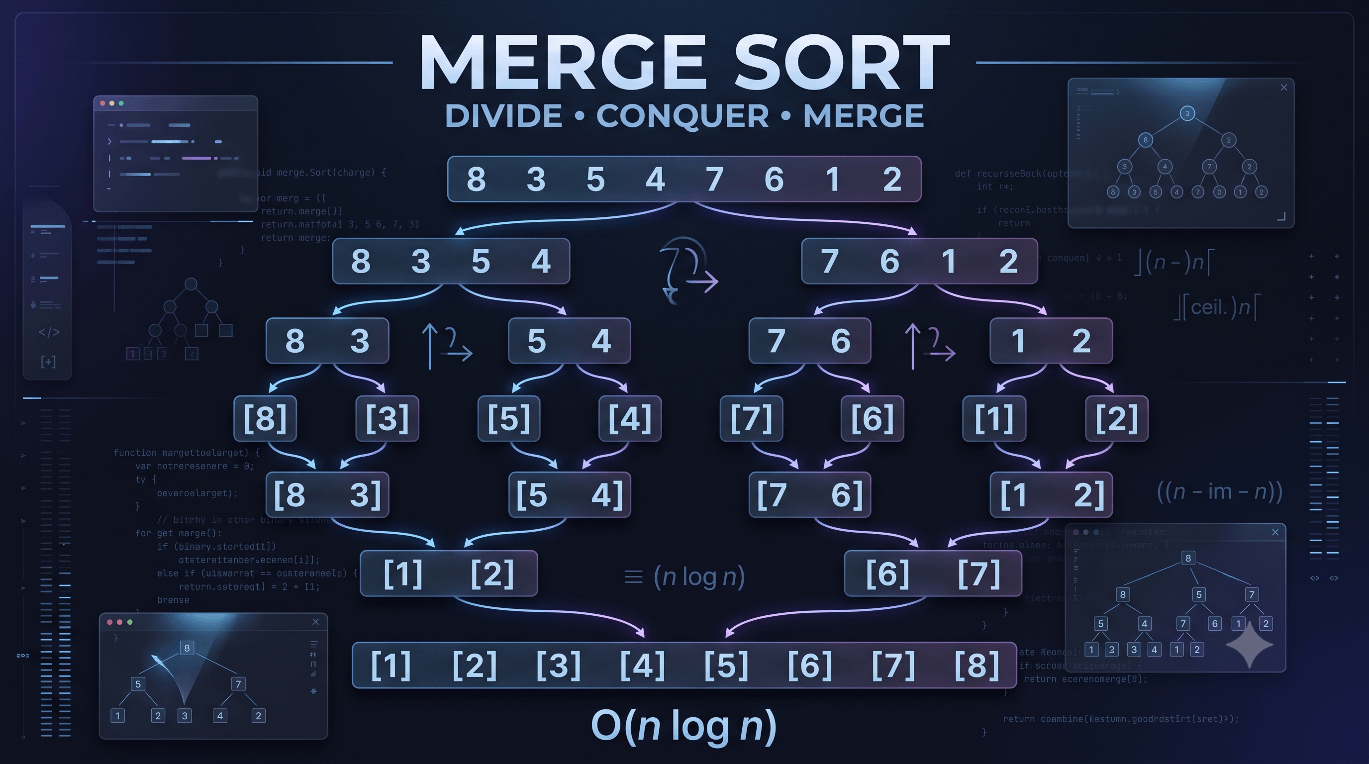
[8, 3, 5, 4, 7, 6, 1, 2]

becomes:

[8, 3, 5, 4]    [7, 6, 1, 2]

Then:

[8, 3] [5, 4]    [7, 6] [1, 2]

Then:

[8] [3] [5] [4] [7] [6] [1] [2]

Now the merging begins.

Why Do We Keep Splitting?

At first, splitting the array may seem pointless.

Why turn:

[8, 3, 5, 4]

into:

[8, 3]
[5, 4]

and then:

[8]
[3]
[5]
[4]

?

Because a single-element array is already sorted.

For example:

[8]

There is nothing to sort.

So instead of directly sorting a complicated array, Merge Sort reduces the problem until it reaches trivial problems.

This is the essence of Divide and Conquer.

Divide and Conquer

Divide and Conquer generally follows three steps:

1. Divide

Break the problem into smaller subproblems.

2. Conquer

Solve the smaller problems.

3. Combine

Combine the solutions into the final answer.

For Merge Sort:

Divide:
[8,3,5,4,7,6,1,2]

↓

Conquer:
Sort smaller arrays

↓

Combine:
Merge sorted arrays

Merge Sort Step by Step

Let's sort:

[8, 3, 5, 4, 7, 6, 1, 2]

Step 1: Divide

Split into two halves:

[8, 3, 5, 4]    [7, 6, 1, 2]

Step 2: Divide Again

[8, 3] [5, 4]    [7, 6] [1, 2]

Step 3: Divide Again

[8] [3] [5] [4] [7] [6] [1] [2]

Now every piece contains exactly one element.

The dividing phase is finished.

Now Comes the Interesting Part: Merging

We now start combining the pieces.

Consider:

[8]
[3]

Both are individually sorted.

Compare:

8 vs 3

3 is smaller.

So:

[3, 8]

Now:

[5]
[4]

Compare:

5 vs 4

Result:

[4, 5]

So our first half becomes:

[3, 8]    [4, 5]

Merging Larger Arrays

Now merge:

[3, 8]
[4, 5]

We compare the first elements.

3 vs 4

Take 3:

[3]

Then:

8 vs 4

Take 4:

[3, 4]

Then:

8 vs 5

Take 5:

[3, 4, 5]

Only 8 remains:

[3, 4, 5, 8]

First half sorted.

Merge the Other Half

We had:

[7, 6]
[1, 2]

First:

[7] + [6]

becomes:

[6, 7]

And:

[1] + [2]

becomes:

[1, 2]

Now merge:

[6, 7]
[1, 2]

Compare:

6 vs 1 → 1
6 vs 2 → 2

Remaining:

6, 7

Result:

[1, 2, 6, 7]

Final Merge

Now we have:

[3, 4, 5, 8]

[1, 2, 6, 7]

Both are sorted.

We merge them.

Compare:

3 vs 1 → 1
3 vs 2 → 2
3 vs 6 → 3
4 vs 6 → 4
5 vs 6 → 5
8 vs 6 → 6
8 vs 7 → 7

Remaining:

8

Final result:

[1, 2, 3, 4, 5, 6, 7, 8]

Sorted!

The Merge Operation

The most important part of Merge Sort is actually the merge operation.

We start with two sorted arrays:

A = [2, 5, 8]
B = [1, 3, 7]

We maintain two pointers:

A → 2
B → 1

Compare:

2 vs 1

Take 1.

Then:

A → 2
B → 3

Compare:

2 vs 3

Take 2.

Continue:

3
5
7
8

Result:

[1, 2, 3, 5, 7, 8]

Why Does Merging Take O(n)?

Suppose the two arrays contain a total of n elements.

Every element is examined and eventually copied into the result.

Therefore:

Merge = O(n)

This fact is crucial to understanding Merge Sort's overall complexity.

Merge Sort Pseudocode

MERGE_SORT(array)

    IF length(array) <= 1
        RETURN array

    middle = length(array) / 2

    left = first half
    right = second half

    left = MERGE_SORT(left)
    right = MERGE_SORT(right)

    RETURN MERGE(left, right)

And the merge function:

MERGE(left, right)

    result = empty array

    WHILE left and right both contain elements

        IF first element of left <= first element of right

            move first element of left to result

        ELSE

            move first element of right to result

    END WHILE

    append remaining elements

    RETURN result

Merge Sort in Python

Here's a clean implementation:

def merge_sort(numbers):

    if len(numbers) <= 1:
        return numbers

    middle = len(numbers) // 2

    left = numbers[:middle]
    right = numbers[middle:]

    left = merge_sort(left)
    right = merge_sort(right)

    return merge(left, right)


def merge(left, right):

    result = []

    i = 0
    j = 0

    while i < len(left) and j < len(right):

        if left[i] <= right[j]:

            result.append(left[i])
            i += 1

        else:

            result.append(right[j])
            j += 1

    result.extend(left[i:])
    result.extend(right[j:])

    return result

Example:

numbers = [8, 3, 5, 4, 7, 6, 1, 2]

sorted_numbers = merge_sort(numbers)

print(sorted_numbers)

Output:

[1, 2, 3, 4, 5, 6, 7, 8]

Understanding the Recursion

Merge Sort uses recursion.

That's why understanding the recursive structure is important.

Consider:

[8, 3, 5, 4]

The function calls itself:

merge_sort([8, 3, 5, 4])
        ↓
merge_sort([8, 3])
        ↓
merge_sort([8])

[8] has one element, so it returns.

Then:

[8] + [3]

are merged.

Then:

[5] + [4]

are merged.

Finally:

[3, 8] + [4, 5]

are merged.

This creates a recursive tree of operations.

Merge Sort Recursion Tree

For:

[8, 3, 5, 4, 7, 6, 1, 2]

the structure looks approximately like:

                 8 3 5 4 7 6 1 2
                 /             \
             8 3 5 4          7 6 1 2
             /     \          /      \
           8 3     5 4      7 6      1 2
           / \     / \      / \      / \
          8   3   5   4    7   6    1   2

Then the results travel upward through the tree:

          [1 2 3 4 5 6 7 8]

This is a beautiful example of recursive problem decomposition.

Why Is Merge Sort O(n log n)?

This is one of the most important questions in DSA interviews.

Let's break it down.

Step 1: How Many Levels?

Every time we divide the array, we approximately halve its size.

For:

n

elements:

n
n/2
n/4
n/8
...
1

The number of levels is:

log₂(n)

Therefore:

Number of levels = O(log n)

Step 2: How Much Work Per Level?

At every level, all elements participate in merging.

So the total work per level is approximately:

O(n)

There are:

O(log n)

levels.

Therefore:

O(n) × O(log n)

equals:

O(n log n)

That's why:

Merge Sort = O(n log n)

Complexity of Merge Sort

Merge Sort has:

Best Case:    O(n log n)
Average Case: O(n log n)
Worst Case:   O(n log n)

This is one of its biggest advantages.

Unlike Quick Sort's basic implementation, Merge Sort doesn't degrade to O(n²) based on unfortunate pivot choices.

Space Complexity

Our Python implementation creates additional arrays.

Therefore:

Auxiliary Space = O(n)

This is the major trade-off.

We get:

Excellent time complexity

but use:

Additional memory

Is Merge Sort Stable?

Yes.

Merge Sort can be implemented as a stable sorting algorithm.

Remember our previous example:

Aman   90
Rahul  90

If the merge operation chooses the left element when values are equal:

if left[i] <= right[j]:

the original relative ordering can be preserved.

This makes Merge Sort useful when sorting structured records.

Merge Sort vs Bubble Sort

Consider:

n = 1,000,000

Bubble Sort:

O(n²)

Merge Sort:

O(n log n)

The difference becomes enormous as n increases.

This is why algorithmic complexity matters.

A program that works perfectly with:

100 records

may become unusable with:

100 million records

if the algorithm doesn't scale.

Merge Sort vs Insertion Sort

Insertion Sort is excellent when:

Small input
Nearly sorted data

Merge Sort is more suitable when:

Large input
Predictable O(n log n)
Stable sorting required

Neither algorithm is universally best.

That's a recurring lesson in software engineering:

There is rarely a single algorithm that is optimal for every situation.

Top-Down Merge Sort

The implementation we've discussed is called Top-Down Merge Sort.

It starts with the entire array:

[8,3,5,4,7,6,1,2]

and recursively divides it:

        Full Array
        /       \
      Half      Half
      / \       / \
    ...       ...

Then merges upward.

Bottom-Up Merge Sort

There is another approach:

Bottom-Up Merge Sort.

Instead of starting with the whole array and recursively splitting, we start with individual elements and iteratively merge them.

Start:

[8] [3] [5] [4] [7] [6] [1] [2]

Merge pairs:

[3,8] [4,5] [6,7] [1,2]

Merge again:

[3,4,5,8] [1,2,6,7]

Finally:

[1,2,3,4,5,6,7,8]

Same fundamental complexity:

O(n log n)

but a different implementation strategy.

Merge Sort in JavaScript

function mergeSort(numbers) {

    if (numbers.length <= 1) {
        return numbers;
    }

    const middle = Math.floor(numbers.length / 2);

    const left = numbers.slice(0, middle);
    const right = numbers.slice(middle);

    return merge(
        mergeSort(left),
        mergeSort(right)
    );
}


function merge(left, right) {

    const result = [];

    let i = 0;
    let j = 0;

    while (i < left.length && j < right.length) {

        if (left[i] <= right[j]) {
            result.push(left[i]);
            i++;
        } else {
            result.push(right[j]);
            j++;
        }
    }

    return result
        .concat(left.slice(i))
        .concat(right.slice(j));
}

Usage:

const numbers = [8, 3, 5, 4, 7, 6, 1, 2];

console.log(mergeSort(numbers));

Output:

[1, 2, 3, 4, 5, 6, 7, 8]

A Common Interview Question

Why doesn't Merge Sort have an O(n²) worst case?

Because its structure doesn't depend on favorable or unfavorable input ordering.

It consistently:

Divide → O(log n) levels
Merge  → O(n) work per level

Therefore:

O(n log n)

in best, average, and worst cases.

Another Interview Question

What is the main disadvantage of Merge Sort?

The primary disadvantage is additional memory.

Typical array-based Merge Sort requires:

O(n)

auxiliary space.

This can matter when memory usage is an important constraint.

Can Merge Sort Work on Linked Lists?

Yes.

Merge Sort is particularly well suited to linked lists because splitting and merging can be performed without requiring random access in the same way array algorithms often do.

This is one reason Merge Sort appears in discussions of linked-list sorting.

Merge Sort in the Real World

The exact sorting algorithm used by a production language or library depends on the implementation and data type.

Modern standard libraries often use sophisticated hybrid algorithms rather than exposing a textbook implementation directly.

But learning Merge Sort gives you an important foundation for understanding:

• Divide and conquer
• Recursion
• Stable sorting
• Complexity analysis
• External sorting
• Large-data processing
• Algorithmic trade-offs

The underlying concepts are much more important than memorizing one implementation.

External Sorting

Here's a fascinating real-world application.

What if your dataset is too large to fit into RAM?

Imagine:

Dataset = 500 GB
RAM = 16 GB

You can't simply load everything into memory and sort it.

One approach is external sorting.

The general idea:

Large Dataset
     ↓
Split into manageable chunks
     ↓
Sort each chunk
     ↓
Store sorted chunks
     ↓
Merge sorted chunks

Notice the familiar pattern?

DIVIDE
+
SORT
+
MERGE

This is closely related to Merge Sort.

This technique is important in large-scale data processing.

The Deeper Lesson

Merge Sort teaches something much more valuable than sorting.

Suppose you have a problem that seems too large:

BIG PROBLEM

Instead of asking:

"How can I solve this giant problem directly?"

ask:

"Can I break it into smaller versions of the same problem?"

Then:

Big Problem
     ↓
Smaller Problems
     ↓
Solve Smaller Problems
     ↓
Combine Results

This pattern appears throughout computer science.

Divide and Conquer Beyond Sorting

The same broad strategy appears in algorithms such as:

• Binary Search
• Merge Sort
• Quick Sort
• Closest Pair of Points
• Strassen's Matrix Multiplication
• Fast Fourier Transform

The specific details differ, but the mindset is similar:

Reduce a difficult problem into manageable pieces.

Common Mistakes in Merge Sort

Mistake 1: Forgetting the Base Case

You need:

if len(numbers) <= 1:
    return numbers

Without a base case, recursion doesn't stop.

Mistake 2: Incorrect Splitting

Make sure the two halves actually cover the entire array.

For example:

left = numbers[:middle]
right = numbers[middle:]

Mistake 3: Forgetting Remaining Elements

During merging, one side may become empty while elements remain on the other side.

You must append them:

result.extend(left[i:])
result.extend(right[j:])

Mistake 4: Incorrect Equality Handling

For stable behavior, using:

left[i] <= right[j]

instead of:

left[i] < right[j]

can preserve the relative ordering of equal elements.

Practice Problem

Try sorting:

[10, 4, 7, 2, 8, 1, 6, 3]

First divide:

[10, 4, 7, 2]    [8, 1, 6, 3]

Then:

[10, 4] [7, 2]    [8, 1] [6, 3]

Then:

[10] [4] [7] [2] [8] [1] [6] [3]

Now manually perform the merging.

The final answer should be:

[1, 2, 3, 4, 6, 7, 8, 10]

Don't skip the merge process.

Understanding how the pointers move is the real exercise.

Merge Sort Cheat Sheet

Algorithm:
Merge Sort

Technique:
Divide and Conquer

Best:
O(n log n)

Average:
O(n log n)

Worst:
O(n log n)

Typical Auxiliary Space:
O(n)

Stable:
Yes, with a suitable implementation

In-place:
Typical array implementation: No

Core Operations:
Divide + Merge

Final Takeaways

Merge Sort is one of the most important algorithms to understand in DSA.

The algorithm follows:

                 ARRAY
                   ↓
                 DIVIDE
                /      \
             LEFT      RIGHT
              ↓          ↓
            SORT       SORT
              \          /
               \        /
                 MERGE
                   ↓
               SORTED ARRAY

The essential ideas are:

• Divide the problem into smaller pieces.
• Continue until each piece is trivially sorted.
• Merge sorted pieces.
• Each level performs O(n) work.
• There are O(log n) levels.
• Therefore total complexity is O(n log n).
• Typical implementations require O(n) auxiliary memory.
• Merge Sort can be stable.
• It demonstrates the power of Divide and Conquer.

And perhaps the most important lesson:

When a problem looks too large, don't always attack it as one giant problem. Break it down.