Heap Sort Explained: Heaps, Heapify & Priority Queues

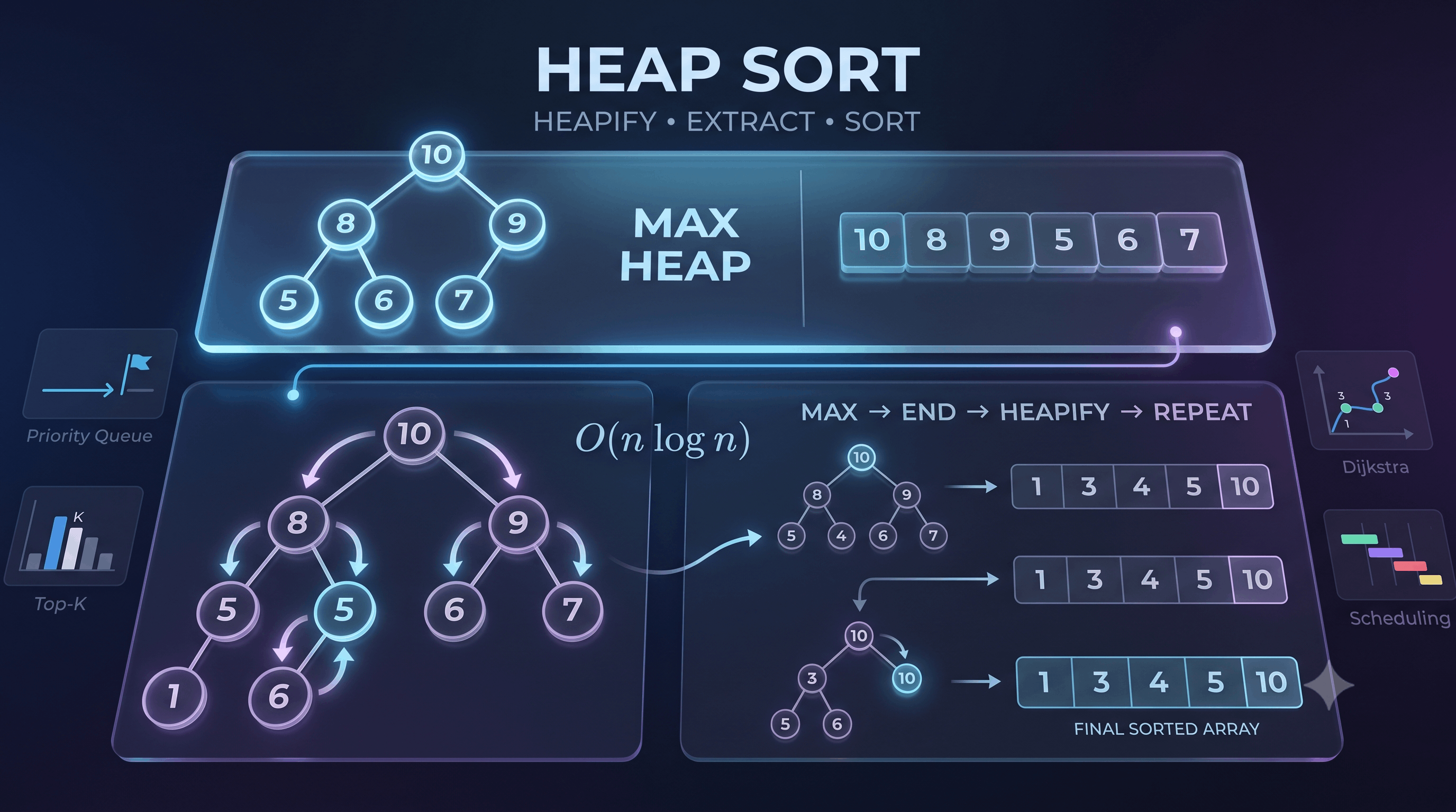
Sorting algorithms have taken us from simple techniques like Bubble Sort to powerful divide-and-conquer algorithms such as Merge Sort and Quick Sort.

Now we're entering another important area of algorithms:

Heaps

A heap is not just a sorting concept.

It is a fundamental data structure used to build:

• Priority Queues
• Scheduling systems
• Graph algorithms
• Top-K problems
• Median-finding algorithms
• Dijkstra's algorithm
• Prim's algorithm
• Heap Sort

In this article, we'll build the concept from the ground up and eventually use it to implement Heap Sort.

What Is a Heap?

A heap is a specialized binary tree that follows a particular ordering property.

There are two primary types:

Min Heap

The smallest element is always at the root.

        1
       / \
      3   5
     / \
    7   9

Here:

parent <= children

Max Heap

The largest element is always at the root.

        9
       / \
      7   8
     / \
    3   5

Here:

parent >= children

For Heap Sort in ascending order, we'll primarily use a Max Heap.

Heap vs Binary Search Tree

This is a common interview question.

A heap and a Binary Search Tree are both binary-tree-based structures, but their rules are different.

A Max Heap guarantees:

parent >= children

A Binary Search Tree generally guarantees:

left subtree < node < right subtree

For example, this is a valid Max Heap:

        10
       /  \
      8    9
     / \
    2   5

But it's not necessarily a Binary Search Tree because the entire left subtree doesn't need to be smaller than the right subtree.

The heap only cares about the parent-child relationship.

The Heap Property

For a Max Heap:

Parent >= Child

For a Min Heap:

Parent <= Child

That's the fundamental rule.

But there is another important requirement.

A binary heap is usually a:

Complete Binary Tree

A complete binary tree fills levels from left to right.

For example:

        10
       /  \
      8    9
     / \  /
    5  6 7

is complete.

But:

        10
       /  \
      8    9
       \
        5

is not complete in the usual heap representation.

Why Are Heaps Usually Stored in Arrays?

Here's something that makes heaps particularly interesting.

We don't need to create a collection of node objects containing pointers to children.

We can store the entire heap in an array.

Consider:

        10
       /  \
      8    9
     / \  /
    5  6 7

Represent it as:

[10, 8, 9, 5, 6, 7]

The tree structure is implied by the indexes.

That's extremely useful.

Heap Index Formulas

For an element at index:

i

using 0-based indexing:

Parent

parent = (i - 1) // 2

Left Child

left = 2 * i + 1

Right Child

right = 2 * i + 2

Let's test this.

Array:

[10, 8, 9, 5, 6, 7]

For:

i = 0

we get:

left  = 1
right = 2

So:

10
├── 8
└── 9

Correct.

For:

i = 1

we get:

left  = 3
right = 4

Therefore:

8
├── 5
└── 6

Exactly.

Why Does This Matter?

Because we can manipulate a tree using simple array indexes.

No explicit tree nodes are required.

This gives heaps excellent memory efficiency.

Building a Max Heap

Consider this array:

[4, 10, 3, 5, 1]

It isn't a Max Heap.

The root is:

4

but its child is:

10

which is larger.

We need to rearrange the elements.

The process used to restore the heap property is called:

Heapify

What Is Heapify?

Heapify means restoring the heap property for a subtree.

Suppose we have:

        4
       / \
      10  3

For a Max Heap, this is invalid:

4 < 10

We compare the node with its children.

The largest value is:

10

So we swap:

        10
       /  \
      4    3

Now the subtree satisfies the Max Heap property.

Heapify Example

Consider:

[4, 10, 3, 5, 1]

Visualized:

        4
       / \
     10   3
    / \
   5   1

Start with node 4.

Children:

10
3

Largest is 10.

Swap:

        10
       /  \
      4    3
     / \
    5   1

But we're not finished.

The 4 moved downward.

Its children are now:

5
1

Since:

5 > 4

swap again:

        10
       /  \
      5    3
     / \
    4   1

Now it's a valid Max Heap.

Array:

[10, 5, 3, 4, 1]

The Heapify Process

Conceptually:

        Node
       /    \
   Left     Right
      \      /
       Largest
          ↓
       Swap
          ↓
      Continue

We continue downward until the heap property is restored.

Heapify Pseudocode

HEAPIFY(array, n, i)

    largest = i

    left = 2*i + 1
    right = 2*i + 2

    IF left < n AND array[left] > array[largest]

        largest = left

    IF right < n AND array[right] > array[largest]

        largest = right

    IF largest != i

        SWAP array[i] and array[largest]

        HEAPIFY(array, n, largest)

The parameter:

n

represents the current heap size.

This becomes particularly important during Heap Sort.

Building the Entire Heap

Now we need to convert an arbitrary array into a Max Heap.

Suppose:

[4, 10, 3, 5, 1]

We don't need to call heapify on every element.

We start from the last non-leaf node.

Why?

Because leaf nodes already satisfy the heap property by themselves.

Finding the Last Non-Leaf Node

For an array of size n, the last non-leaf node is:

(n // 2) - 1

For:

n = 5

we get:

(5 // 2) - 1
= 2 - 1
= 1

So we start at index:

1

Then move backward:

1
0

Heapify each node.

Build Heap Example

Start:

[4, 10, 3, 5, 1]

Heapify index 1.

Subtree:

      10
     /  \
    5    1

Already valid.

Array remains:

[4, 10, 3, 5, 1]

Now heapify index 0.

Subtree:

        4
       / \
     10   3

Largest is 10.

Swap:

[10, 4, 3, 5, 1]

Continue heapifying the 4:

      4
     / \
    5   1

Swap:

[10, 5, 3, 4, 1]

We now have a Max Heap.

The Most Important Idea in Heap Sort

Once we have:

[10, 5, 3, 4, 1]

the largest element is guaranteed to be at:

index 0

That's exactly what Heap Sort needs.

We can repeatedly remove the maximum element.

Heap Sort Step by Step

Suppose:

[4, 10, 3, 5, 1]

Build a Max Heap:

[10, 5, 3, 4, 1]

Now:

10

is the largest element.

Swap it with the last element:

[1, 5, 3, 4, 10]

We've placed 10 in its final position.

But the remaining heap:

[1, 5, 3, 4]

is no longer a Max Heap.

So we heapify again:

[5, 4, 3, 1, 10]

Now swap the maximum with the last element of the active heap:

[1, 4, 3, 5, 10]

Heapify:

[4, 1, 3, 5, 10]

Continue.

Eventually:

[1, 3, 4, 5, 10]

Sorted.

The Heap Sort Pattern

The algorithm is essentially:

Build Max Heap
     ↓
Move maximum to the end
     ↓
Reduce heap size
     ↓
Heapify
     ↓
Move next maximum to the end
     ↓
Repeat

The important trick is:

The sorted portion grows from the right side of the array.

Heap Sort Pseudocode

HEAP_SORT(array)

    n = length(array)

    BUILD_MAX_HEAP(array)

    FOR end = n - 1 DOWN TO 1

        SWAP array[0] and array[end]

        HEAPIFY(array, end, 0)

Build heap:

BUILD_MAX_HEAP(array)

    n = length(array)

    FOR i = (n // 2) - 1 DOWN TO 0

        HEAPIFY(array, n, i)

Heap Sort in Python

def heapify(numbers, n, i):

    largest = i

    left = 2 * i + 1
    right = 2 * i + 2

    if left < n and numbers[left] > numbers[largest]:
        largest = left

    if right < n and numbers[right] > numbers[largest]:
        largest = right

    if largest != i:

        numbers[i], numbers[largest] = (
            numbers[largest],
            numbers[i]
        )

        heapify(numbers, n, largest)


def heap_sort(numbers):

    n = len(numbers)

    # Build Max Heap
    for i in range(n // 2 - 1, -1, -1):
        heapify(numbers, n, i)

    # Extract maximum elements
    for end in range(n - 1, 0, -1):

        numbers[0], numbers[end] = (
            numbers[end],
            numbers[0]
        )

        heapify(numbers, end, 0)


numbers = [4, 10, 3, 5, 1]

heap_sort(numbers)

print(numbers)

Output:

[1, 3, 4, 5, 10]

Why Does Heap Sort Work?

At every iteration:

array[0]

contains the largest element in the active heap.

We move it to the end:

[largest]

That position is now permanently sorted.

Then we reduce the heap size.

For example:

[10, 5, 3, 4, 1]

After extracting 10:

[1, 5, 3, 4 | 10]

The vertical bar represents:

heap | sorted

Then:

[5, 4, 3, 1 | 10]

Extract 5:

[1, 4, 3 | 5, 10]

Eventually:

[1, 3, 4, 5, 10]

Heap Sort Complexity

Let's analyze it carefully.

Building the heap takes:

O(n)

Then we perform approximately n extraction operations.

Each extraction requires heapifying:

O(log n)

Therefore:

n × log n

gives:

O(n log n)

So Heap Sort has:

Best Case:    O(n log n)
Average Case: O(n log n)
Worst Case:   O(n log n)

This predictable worst-case performance is a major advantage.

Space Complexity

A typical in-place Heap Sort implementation uses:

O(1)

auxiliary space apart from the recursion stack if heapify is implemented recursively.

An iterative heapify implementation can achieve:

O(1)

auxiliary space.

This is one of Heap Sort's biggest advantages over a typical Merge Sort implementation.

Is Heap Sort Stable?

Generally:

No

Heap Sort is not a stable sorting algorithm.

If two records have equal keys, their relative order may change during heap operations.

Heap Sort Cheat Sheet

Algorithm:
Heap Sort

Data Structure:
Binary Heap

Technique:
Heapify + Repeated Extraction

Best:
O(n log n)

Average:
O(n log n)

Worst:
O(n log n)

Auxiliary Space:
O(1) with iterative heapify

Stable:
No

In-place:
Yes

Typical Heap:
Max Heap for ascending sort

Why Is Heapify O(log n)?

A heap is a complete binary tree.

For n elements, its height is:

O(log n)

During heapify, an element may travel from the root toward the bottom.

Therefore the maximum number of levels it can travel is:

O(log n)

Hence:

Heapify = O(log n)

Why Is Building a Heap O(n)?

This is a classic interview question.

You might initially think:

n elements × O(log n)

which would give:

O(n log n)

But bottom-up heap construction actually takes:

O(n)

Why?

Because most nodes are near the bottom and can move only a very small distance.

Only a few nodes are near the top and can travel many levels.

The total work across all nodes adds up to linear time.

This is an excellent example of why simply multiplying:

number of operations × worst-case cost

can sometimes give an overly loose bound.

Priority Queue

Now we arrive at one of the most important applications of heaps.

A Priority Queue is a data structure where elements are processed according to priority rather than simply arrival order.

Imagine:

Emergency Room

Patients don't necessarily get treated in the order they arrive.

A higher-priority case may be handled first.

A priority queue models this idea.

Priority Queue Using a Heap

Suppose we have:

Task A → Priority 3
Task B → Priority 10
Task C → Priority 5
Task D → Priority 1

A Max Heap can keep the highest priority at the root:

        10
       /  \
      3    5
     /
    1

The next task to process is immediately available at the root.

Heap Operations

A heap supports several important operations.

Insert

Add an element and restore the heap property.

Typically:

O(log n)

Extract Max

Remove the largest element from a Max Heap.

Typically:

O(log n)

Extract Min

For a Min Heap:

O(log n)

Peek

Look at the minimum or maximum element without removing it.

Typically:

O(1)

Heap vs Sorted Array

Suppose you need to repeatedly retrieve the largest element.

With a sorted array:

[1, 2, 3, 4, 5, 6, 7]

the maximum is easy to find.

But inserting a new element while maintaining sorting can be expensive.

A heap provides a better balance:

Peek max       O(1)
Insert         O(log n)
Extract max    O(log n)

This is why heaps are ideal for priority queues.

Heap Applications

Heaps appear throughout computer science.

1. Priority Queues

Task scheduling, job processing, event systems.

2. Dijkstra's Algorithm

Efficiently selecting the next closest vertex.

3. Prim's Algorithm

Efficiently selecting the next minimum-cost edge.

4. Top-K Problems

Finding:

Top 10 largest elements
Top 10 smallest elements

without necessarily sorting the entire dataset.

5. Scheduling

Operating systems and distributed systems can use priority-based scheduling concepts.

6. Median Finding

Two heaps can be combined to maintain a running median efficiently.

The Top-K Pattern

This is one of the most useful heap patterns for interviews.

Suppose you have:

10 million numbers

and want:

10 largest numbers

A naive approach is:

Sort all 10 million numbers

That costs approximately:

O(n log n)

But if you only need 10 values, a heap can be much more efficient.

Maintain a Min Heap of size k:

k = 10

As you scan the numbers:

If heap size < 10:
    insert

Else if current > minimum:
    remove minimum
    insert current

Complexity:

O(n log k)

Since k is only 10, this can be significantly cheaper than sorting everything.

Two Heaps for Median

Another powerful technique is using two heaps.

Maintain:

Max Heap → smaller half
Min Heap → larger half

Conceptually:

        Smaller Half
        Max Heap
           ↓
[10, 20, 30]

[40, 50, 60]
           ↑
        Min Heap
        Larger Half

The middle values remain near the roots.

This allows us to calculate a running median efficiently.

This pattern appears frequently in advanced interview questions.

Heap vs Stack vs Queue

These data structures solve different problems.

A heap is therefore not simply "another queue."

It's a data structure that can efficiently implement priority-based retrieval.

Common Heap Mistakes

Mistake 1: Confusing Heap With BST

A heap does not guarantee:

left < parent < right

It only guarantees the heap property.

Mistake 2: Forgetting Complete Tree Structure

A binary heap must maintain its complete-tree structure.

Mistake 3: Using the Wrong Child Formula

For 0-based arrays:

left  = 2*i + 1
right = 2*i + 2

Memorize these.

Mistake 4: Heapifying the Wrong Range

During Heap Sort, after moving the maximum to the end:

[heap | sorted]

the sorted portion must no longer be considered part of the heap.

That's why we pass a smaller heap size to heapify.

Interview Questions

What is a heap?

A complete binary tree satisfying a heap-order property.

What is a Max Heap?

A heap where every parent is greater than or equal to its children.

What is a Min Heap?

A heap where every parent is less than or equal to its children.

What is Heap Sort complexity?

O(n log n)

in best, average, and worst cases.

Is Heap Sort stable?

No, not generally.

Is Heap Sort in-place?

Yes, typical array implementations are.

What is heapify complexity?

O(log n)

What is building a heap complexity?

O(n)

What is the root of a Max Heap?

The maximum element.

What is the root of a Min Heap?

The minimum element.

A Classic Interview Problem

Given:

[3, 2, 1, 5, 6, 4]

find the:

2nd largest element

A simple approach is:

Sort

Result:

[1, 2, 3, 4, 5, 6]

Answer:

5

But if the array is huge, sorting everything may be unnecessary.

A heap-based approach can maintain only the elements required for the answer.

This is the beginning of a much larger family of problems:

Top-K Problems

We'll explore those later in this series.

Heap Sort vs Quick Sort vs Merge Sort

There is no universally superior algorithm.

Each represents a different engineering trade-off.

Practice Problem

Build a Max Heap from:

[3, 9, 2, 1, 4, 5]

Try doing it manually.

Start from:

index = (n // 2) - 1

Then heapify toward index 0.

After building the Max Heap, perform Heap Sort.

Your final sorted array should be:

[1, 2, 3, 4, 5, 9]

But don't just verify the answer.

The important exercise is understanding why every swap happens.

The Bigger Picture

So far, our algorithm journey looks like:

Searching
   ↓
Linear Search
   ↓
Binary Search

Sorting
   ↓
Bubble Sort
   ↓
Selection Sort
   ↓
Insertion Sort
   ↓
Merge Sort
   ↓
Quick Sort
   ↓
Heap Sort

Notice how the concepts are becoming more sophisticated.

We started with:

Compare

Then:

Divide and Conquer

Then:

Partition

And now:

Hierarchical Data Structure

This is exactly how your algorithmic thinking should develop.

Final Takeaways

Heap Sort teaches us much more than sorting.

The key concepts are:

• A heap is a complete binary tree.
• A Max Heap keeps the maximum at the root.
• A Min Heap keeps the minimum at the root.
• Heaps are commonly represented using arrays.
• left = 2i + 1
• right = 2i + 2
• Heapify restores the heap property.
• Building a heap takes O(n).
• Heap Sort takes O(n log n).
• Typical Heap Sort is in-place.
• Heap Sort is generally not stable.
• Heaps power priority queues.
• Heaps are extremely useful for Top-K problems.
• Two heaps can solve running-median problems.

The most important mental model is:

              HEAP
                ↓
        Maximum / Minimum
                ↓
       Efficient Retrieval
                ↓
     Priority Queue / Sorting
                ↓
        Advanced Algorithms

Once you understand heaps, a large number of advanced DSA problems become much easier to recognize.