Counting Sort Explained: Frequency Arrays, Prefix Sums & When It Beats Quick Sort

Introduction

When learning sorting algorithms, we usually encounter algorithms such as:

• Bubble Sort
• Selection Sort
• Insertion Sort
• Merge Sort
• Quick Sort
• Heap Sort

Most of these algorithms compare elements with each other.

For example:

5 > 3
8 > 2
4 < 7

This leads to an important theoretical limitation: comparison-based sorting algorithms cannot generally do better than Ω(n log n) in the comparison model.

But what if we don't compare the elements at all?

What if we use the values themselves as information to determine where elements belong?

That's exactly the idea behind Counting Sort.

Counting Sort can sort certain integer datasets in:

O(n + k)

where:

• n = number of elements
• k = range of values

When k is reasonably small, Counting Sort can be remarkably fast.

In this article, we'll understand Counting Sort from the ground up, implement it in Python, make it stable, handle negative numbers, understand prefix sums, and see why Counting Sort is an important building block for Radix Sort.

1. What Is Counting Sort?

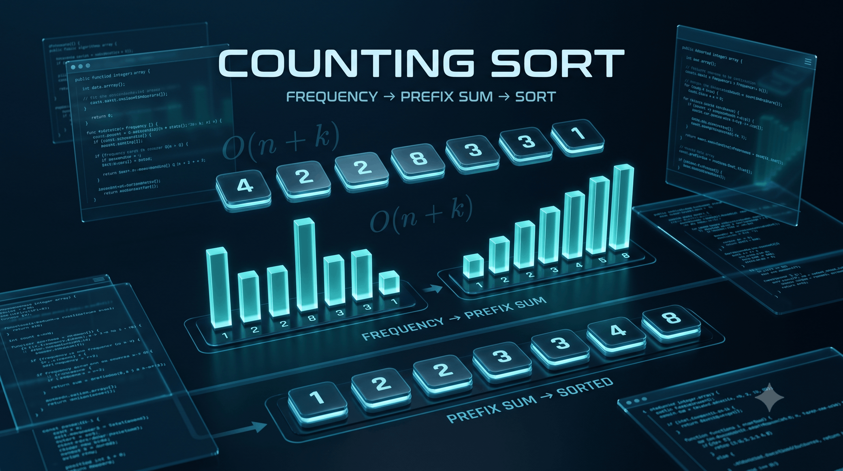
Counting Sort is a non-comparison-based sorting algorithm that sorts integers by counting how many times each value occurs.

Instead of asking:

Is 7 greater than 4?

Counting Sort asks:

How many 4s are there?

How many 5s are there?

How many 6s are there?

And so on.

Consider:

[4, 2, 2, 8, 3, 3, 1]

We can count the occurrences:

1 → 1
2 → 2
3 → 2
4 → 1
5 → 0
6 → 0
7 → 0
8 → 1

Now we simply reconstruct the array:

[1, 2, 2, 3, 3, 4, 8]

No element-to-element comparisons were required.

2. Why Is Counting Sort Different?

Consider Quick Sort.

Quick Sort repeatedly performs comparisons:

5 < 8
2 < 5
7 > 5

Merge Sort does the same:

3 < 8
4 > 2

Counting Sort works differently.

For:

[4, 2, 2, 8, 3, 3, 1]

it creates a frequency table.

Value:   1 2 3 4 5 6 7 8
Count:   1 2 2 1 0 0 0 1

The counts directly tell us how many copies of each value should appear.

That's why Counting Sort is called a non-comparison sorting algorithm.

3. The Core Idea

Counting Sort follows a simple process.

Step 1: Find the range

Find:

minimum value
maximum value

For:

[4, 2, 2, 8, 3, 3, 1]

we have:

min = 1
max = 8

Therefore:

range = 8 - 1 + 1 = 8

Step 2: Create a count array

Create an array of size 8:

count = [0, 0, 0, 0, 0, 0, 0, 0]

Step 3: Count every value

Process the input:

4
2
2
8
3
3
1

The count array becomes:

Index:  0 1 2 3 4 5 6 7
Value:  1 2 3 4 5 6 7 8
Count:  1 2 2 1 0 0 0 1

Step 4: Reconstruct the sorted array

Read the count array from left to right.

1 → once
2 → twice
3 → twice
4 → once
8 → once

Result:

[1, 2, 2, 3, 3, 4, 8]

That's Counting Sort.

4. A Complete Example

Let's take:

arr = [4, 2, 2, 8, 3, 3, 1]

Initial array

4 2 2 8 3 3 1

Frequency table

1 → 1
2 → 2
3 → 2
4 → 1
5 → 0
6 → 0
7 → 0
8 → 1

Reconstruct

1
2 2
3 3
4
8

Final:

[1, 2, 2, 3, 3, 4, 8]

5. Basic Counting Sort Implementation

Here is the simplest implementation in Python:

def counting_sort(arr):
    if not arr:
        return arr

    min_value = min(arr)
    max_value = max(arr)

    count = [0] * (max_value - min_value + 1)

    # Count occurrences
    for num in arr:
        count[num - min_value] += 1

    # Reconstruct sorted array
    index = 0

    for i, frequency in enumerate(count):
        value = i + min_value

        for _ in range(frequency):
            arr[index] = value
            index += 1

    return arr


arr = [4, 2, 2, 8, 3, 3, 1]

print(counting_sort(arr))

Output:

[1, 2, 2, 3, 3, 4, 8]

6. Why Do We Use num - min_value?

You may have noticed:

count[num - min_value] += 1

Why not:

count[num] += 1

Because the minimum value doesn't necessarily have to be 0.

Suppose:

arr = [10, 12, 11, 10]

Then:

min = 10
max = 12

The required range is:

10, 11, 12

We only need three positions.

We map:

10 → 0
11 → 1
12 → 2

using:

index = value - min

Therefore:

10 - 10 = 0
11 - 10 = 1
12 - 10 = 2

This makes the algorithm work efficiently even when the values don't start from zero.

7. Handling Negative Numbers

Counting Sort can also handle negative integers if we use an offset.

Consider:

[-5, -2, -5, 0, 3, -1]

Minimum:

-5

Maximum:

3

Range:

3 - (-5) + 1 = 9

Mapping becomes:

-5 → 0
-4 → 1
-3 → 2
-2 → 3
-1 → 4
 0 → 5
 1 → 6
 2 → 7
 3 → 8

The same formula works:

index = num - min_value

Implementation:

def counting_sort(arr):
    if not arr:
        return arr

    min_value = min(arr)
    max_value = max(arr)

    count = [0] * (max_value - min_value + 1)

    for num in arr:
        count[num - min_value] += 1

    index = 0

    for i, frequency in enumerate(count):
        value = i + min_value

        for _ in range(frequency):
            arr[index] = value
            index += 1

    return arr


arr = [-5, -2, -5, 0, 3, -1]

print(counting_sort(arr))

Output:

[-5, -5, -2, -1, 0, 3]

8. The Most Important Concept: Range

Counting Sort's performance depends heavily on the range of values.

Suppose:

arr = [1, 2, 3, 4, 5]

Here:

n = 5
k = 5

Excellent.

But consider:

arr = [1, 1000000000]

There are only two elements.

n = 2

But:

k = 1,000,000,000

Creating:

[0, 0, 0, 0, 0, ...]

with one billion positions would be extremely wasteful.

This gives us one of the most important rules for Counting Sort:

Counting Sort is efficient when the value range is not much larger than the number of elements.

9. Time Complexity

Counting Sort has:

O(n + k)

time complexity.

Where:

• n = number of input elements
• k = range of values

Why?

We perform operations involving:

n

input elements.

And we process:

k

possible values.

Therefore:

O(n + k)

10. Is Counting Sort Faster Than O(n log n)?

Potentially, yes.

Suppose:

n = 1,000,000
k = 1,000

Counting Sort performs roughly:

O(1,001,000)

scale operations.

A comparison sort would typically be around:

O(n log n)

which is substantially larger.

But this does not mean Counting Sort is always faster.

If:

n = 1,000
k = 1,000,000,000

Counting Sort becomes impractical.

So algorithm selection depends on the relationship between:

n

and:

k

11. Space Complexity

The basic version requires a count array of size k.

Therefore:

Space = O(k)

If we use the stable version, we typically also create an output array of size n.

Then:

Space = O(n + k)

12. Is Counting Sort Stable?

The simple reconstruction version we wrote is not generally considered a stable sorting implementation because it doesn't preserve the relative ordering of equal elements when sorting records.

For example, imagine:

[
    (2, "A"),
    (1, "B"),
    (2, "C")
]

A stable sort must produce:

(1, "B")
(2, "A")
(2, "C")

Notice:

A

remains before:

C

because both have key 2.

To achieve this, we use cumulative counts and an output array.

This is one of the most important versions of Counting Sort.

13. Prefix Sums in Counting Sort

Suppose we have:

arr = [4, 2, 2, 8, 3, 3, 1]

Frequency counts:

Value:  1 2 3 4 5 6 7 8
Count:  1 2 2 1 0 0 0 1

Now calculate cumulative counts:

Value:       1 2 3 4 5 6 7 8
Frequency:   1 2 2 1 0 0 0 1
Cumulative:  1 3 5 6 6 6 6 7

The cumulative count tells us the final position boundary of each value.

For example:

1 → position 1
2 → position 3
3 → position 5
4 → position 6
8 → position 7

This lets us place every element into its correct position.

14. Stable Counting Sort Implementation

def counting_sort(arr):
    if not arr:
        return arr

    min_value = min(arr)
    max_value = max(arr)

    k = max_value - min_value + 1

    count = [0] * k

    # Step 1: Count frequencies
    for num in arr:
        count[num - min_value] += 1

    # Step 2: Convert counts to cumulative counts
    for i in range(1, k):
        count[i] += count[i - 1]

    # Step 3: Build output array
    output = [0] * len(arr)

    for num in reversed(arr):
        index = num - min_value
        output[count[index] - 1] = num
        count[index] -= 1

    return output


arr = [4, 2, 2, 8, 3, 3, 1]

print(counting_sort(arr))

Output:

[1, 2, 2, 3, 3, 4, 8]

15. Why Do We Traverse Backward?

This line is critical:

for num in reversed(arr):

Why?

Because when multiple elements have the same key, processing from right to left preserves their original relative order.

That is what gives us stability.

This technique becomes particularly important when Counting Sort is used inside Radix Sort.

16. Counting Sort vs Quick Sort

Let's compare them.

Counting Sort can outperform Quick Sort when:

k ≈ O(n)

and the data consists of suitable integer keys.

17. Counting Sort vs Merge Sort

Merge Sort is more general.

Counting Sort is more specialized.

18. Counting Sort vs Heap Sort

19. Real-World Applications

Counting Sort is useful when the possible values are limited.

Example 1: Exam Scores

Suppose students receive scores from:

0 to 100

Even if there are:

1,000,000 students

the range is only:

101

Counting Sort can be extremely effective.

Example 2: Ages

If you're sorting people's ages:

0 to 120

the range is tiny.

A frequency array is an obvious solution.

Example 3: Product Ratings

Suppose ratings are:

1, 2, 3, 4, 5

Counting frequencies is very efficient.

Example 4: Character Frequencies

Counting techniques are widely useful when processing:

letters
digits
small integer IDs
categorical values

20. Counting Sort and Histograms

There is a strong connection between Counting Sort and histograms.

A histogram answers:

How many times does each value occur?

Counting Sort uses exactly this information.

For example:

Data:

1 2 2 3 3 3 4 5

Frequency:

1 → █
2 → ██
3 → ███
4 → █
5 → █

This is essentially the same information required by Counting Sort.

21. Why Counting Sort Matters for Radix Sort

Counting Sort becomes even more interesting when we move toward advanced algorithms.

Consider a number:

329

We can break it into digits:

3
2
9

Radix Sort sorts numbers digit by digit.

For each digit position, it commonly uses a stable Counting Sort.

For example:

170
045
075
090
802
024
002
066

Radix Sort processes:

ones digit
↓
tens digit
↓
hundreds digit

Stable Counting Sort makes this possible.

So learning Counting Sort isn't just learning one algorithm.

It prepares us for:

Radix Sort

which is the next major step in this sorting-algorithm journey.

22. A Common Interview Trap

An interviewer might ask:

"Counting Sort is O(n + k). Therefore, is it always faster than Quick Sort's O(n log n)?"

The correct answer is:

No.

Because k matters.

Suppose:

n = 100
k = 1,000,000,000

Then:

O(n + k)

is enormous.

Meanwhile, Quick Sort can operate efficiently without allocating a billion-element count array.

So you should never look at only:

O(n)

or:

O(n log n)

without considering the assumptions behind the algorithm.

23. Interview Questions

Question 1

Is Counting Sort comparison-based?

No.

It uses the values of elements as indexes into a frequency structure.

Question 2

What is the time complexity?

O(n + k)

where k is the value range.

Question 3

When is Counting Sort efficient?

When:

k

is reasonably small relative to:

n

Question 4

Can Counting Sort handle negative numbers?

Yes.

Use an offset based on the minimum value:

index = num - min_value

Question 5

Is Counting Sort stable?

A Counting Sort implementation can be stable.

The stable version uses:

• cumulative counts
• an output array
• reverse traversal of the input

Question 6

Why is stability important?

Stability matters when sorting records by multiple keys.

For example:

Sort employees by department
then by salary

A stable sorting algorithm can preserve the ordering established by a previous sort.

Question 7

Can Counting Sort sort strings directly?

Not in its basic form.

However, Counting Sort can be used to sort characters or fixed-position digits, which is one reason it is useful in algorithms such as Radix Sort.

24. Common Mistakes

Mistake 1: Ignoring the range

Don't assume:

O(n + k)

is automatically better than:

O(n log n)

Always consider k.

Mistake 2: Creating a gigantic frequency array

Avoid:

[1, 1,000,000,000]

with a billion-sized count array.

The data is sparse, and Counting Sort is a poor choice.

Mistake 3: Forgetting negative values

If negative numbers are possible, don't directly use:

count[num]

Use an offset.

Mistake 4: Assuming every implementation is stable

A frequency-based reconstruction implementation is not automatically stable.

If stability is required, use cumulative counts and an output array.

25. When Should You Use Counting Sort?

Counting Sort is a strong choice when:

✓ Data consists of integers
✓ Range of values is known or reasonably small
✓ k is not dramatically larger than n
✓ You need predictable linear-style performance
✓ Frequencies are useful

Avoid it when:

✗ Values have a massive range
✗ Data is sparse across a huge key space
✗ Elements are arbitrary objects
✗ Memory is severely constrained

26. A Practical Decision-Making Example

Suppose you have:

10 million exam scores

where each score is between:

0 and 100

Counting Sort is an excellent candidate.

Why?

n = 10,000,000
k = 101

The range is tiny compared with the dataset.

Now imagine:

10 million transaction IDs

where IDs range from:

1 to 10 billion

Counting Sort would be a poor choice.

The key lesson is:

Don't choose an algorithm only by its Big-O expression. Understand the parameters behind that expression.

27. Counting Sort in One Picture

The entire algorithm can be remembered as:

INPUT
  ↓
Find MIN and MAX
  ↓
Create COUNT ARRAY
  ↓
Count frequencies
  ↓
Cumulative counts (stable version)
  ↓
Place elements
  ↓
SORTED OUTPUT

Or simply:

VALUES
  ↓
FREQUENCY
  ↓
PREFIX SUM
  ↓
POSITIONS
  ↓
SORTED ARRAY

28. The Bigger Algorithmic Picture

So far in our sorting journey, we've moved through:

Bubble Sort
     ↓
Selection Sort
     ↓
Insertion Sort
     ↓
Merge Sort
     ↓
Quick Sort
     ↓
Heap Sort
     ↓
Counting Sort

We've now crossed an important boundary.

Earlier algorithms primarily relied on comparisons.

Counting Sort shows us another paradigm:

Use additional information about the input to avoid comparisons.

This idea appears repeatedly in advanced computer science.

29. Practice Problems

Before moving forward, try implementing these yourself.

Problem 1

Sort:

[4, 2, 2, 8, 3, 3, 1]

using Counting Sort.

Problem 2

Sort an array containing negative numbers:

[-4, -1, -3, 2, 0, -1]

Problem 3

Find the most frequent element using a frequency array.

Example:

[1, 3, 2, 3, 4, 3, 2]

Expected:

3

Problem 4

Given student scores between 0 and 100, sort them efficiently.

Think about why Counting Sort is a particularly good choice.

Problem 5

Implement stable Counting Sort for records:

[
    (2, "A"),
    (1, "B"),
    (2, "C"),
    (1, "D")
]

Your result should preserve the relative order of equal keys.

30. Key Takeaways

Remember these points for interviews:

Counting Sort
    ↓
Non-comparison sorting
    ↓
Uses frequencies
    ↓
Time = O(n + k)
    ↓
Space = O(k)
    ↓
Stable version = O(n + k) space
    ↓
Excellent for small integer ranges
    ↓
Poor for huge sparse ranges
    ↓
Can handle negative numbers using an offset
    ↓
Prefix sums enable stable placement
    ↓
Foundation for Radix Sort

The most important concept is not simply memorizing:

O(n + k)

Instead, understand why k matters.

That's the difference between memorizing algorithms and actually knowing when to use them.