Machine Learning Model Evaluation: Accuracy, Precision, Recall, F1-Score & More

Building a Machine Learning model is only half the job.

The next question is much more important:

How do we know whether the model is actually good?

Suppose you train a model that predicts whether a customer will purchase a product.

The model reports:

95% accuracy.

Sounds impressive.

But what if only 1% of your customers actually purchase?

The model could predict "No Purchase" for everyone and still achieve approximately 99% accuracy.

Suddenly, that 95% number doesn't tell the whole story.

This is why Machine Learning requires model evaluation metrics.

Different problems require different ways of measuring performance.

For classification problems, we may use:

• Accuracy
• Precision
• Recall
• F1-score
• Specificity
• ROC-AUC
• PR-AUC
• Log loss

For regression problems, we commonly use:

• MAE
• MSE
• RMSE
• R²
• MAPE

Understanding these metrics is essential for building reliable Machine Learning systems.

Table of Contents

1. What Is Model Evaluation?
2. Why Accuracy Isn't Enough
3. Training vs Validation vs Test Performance
4. Confusion Matrix
5. True Positive
6. True Negative
7. False Positive
8. False Negative
9. Accuracy
10. Precision
11. Recall
12. F1-Score
13. Precision vs Recall
14. Specificity
15. ROC-AUC
16. PR-AUC
17. Log Loss
18. Regression Metrics
19. MAE
20. MSE
21. RMSE
22. R²
23. Choosing the Right Metric
24. Common Evaluation Mistakes
25. Real-World Examples
26. Frequently Asked Questions
27. Key Takeaways
28. Conclusion

What Is Model Evaluation?

Model evaluation is the process of measuring how well a Machine Learning model performs on data that represents the conditions in which it will be used.

The evaluation process helps answer questions such as:

• Is the model accurate?
• Does it generalize?
• Does it make too many false alarms?
• Does it miss important cases?
• Is it reliable across different groups?
• Is its performance good enough for deployment?

The right metric depends heavily on the problem.

Why Accuracy Isn't Enough

Let's consider a fraud detection system.

Suppose you have:

100,000 transactions

Only:

500 transactions are fraudulent

That means:

99,500 → Legitimate

500 → Fraud

Now imagine a useless model that predicts:

Every transaction → Legitimate

It gets:

99,500 / 100,000 = 99.5%

accuracy.

That's excellent accuracy.

But the model detects:

0 fraudulent transactions

In a fraud detection system, that model is practically useless.

This is why class imbalance makes accuracy particularly misleading.

Training, Validation, and Test Performance

Before discussing individual metrics, remember that evaluation should generally happen on data that wasn't used to fit the model.

A typical workflow is:

Dataset

   ↓

Training Data

   ↓

Model Training

   ↓

Validation Data

   ↓

Model Selection / Tuning

   ↓

Test Data

   ↓

Final Evaluation

The test set should ideally be treated as an independent final check.

The Confusion Matrix

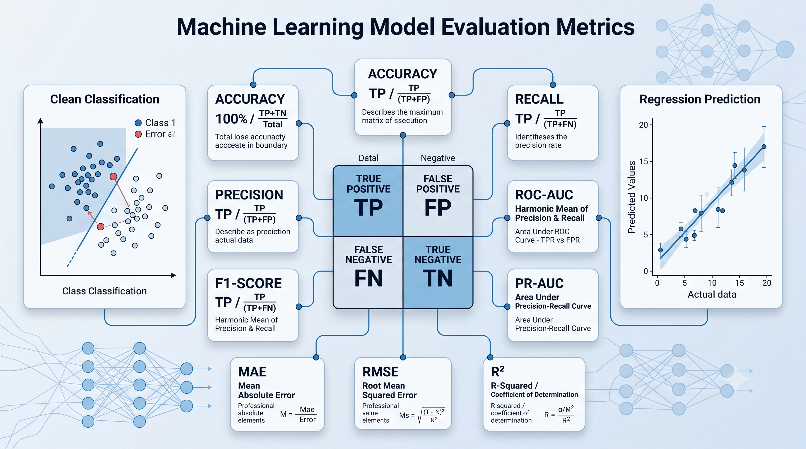
For binary classification, one of the most important evaluation tools is the confusion matrix.

It compares:

Actual values

with

Predicted values.

The four fundamental outcomes are:

Let's understand each one.

True Positive — TP

A True Positive occurs when:

The model predicts positive, and the actual result is positive.

Example:

Actual: Fraud

Prediction: Fraud

Correct.

True Negative — TN

A True Negative occurs when:

The model predicts negative, and the actual result is negative.

Example:

Actual: Legitimate

Prediction: Legitimate

Correct.

False Positive — FP

A False Positive occurs when:

The model predicts positive, but the actual result is negative.

Example:

Actual: Legitimate

Prediction: Fraud

This is sometimes called a false alarm.

False Negative — FN

A False Negative occurs when:

The model predicts negative, but the actual result is positive.

Example:

Actual: Fraud

Prediction: Legitimate

This can be particularly costly in applications where missing a positive case is dangerous.

Visualizing the Confusion Matrix

                    ACTUAL

              Positive    Negative

PREDICTED

Positive        TP          FP

Negative        FN          TN

Almost every common binary classification metric can be derived from these four numbers.

Accuracy

Accuracy measures the proportion of predictions that are correct.

The formula is:

Accuracy =

(TP + TN)

----------------

(TP + TN + FP + FN)

For example:

TP = 80

TN = 90

FP = 10

FN = 20

Then:

Accuracy = (80 + 90) / 200

         = 85%

When Is Accuracy Useful?

Accuracy can be useful when:

• Classes are reasonably balanced
• False positives and false negatives have similar consequences
• The cost of different errors is not dramatically different

For balanced classification problems, accuracy can be a useful summary.

But it should not automatically be the primary metric for every classification problem.

Precision

Precision measures how many of the cases predicted as positive were actually positive.

The formula is:

Precision =

TP

---------

TP + FP

Suppose:

TP = 80

FP = 20

Then:

Precision = 80 / 100

          = 80%

In simple terms:

When the model says "Positive", how often is it correct?

Example of Precision

Imagine an email spam detector.

The model marks 100 emails as spam.

Of those:

80 → Actually Spam

20 → Actually Legitimate

Precision:

80 / 100 = 80%

A higher precision means fewer legitimate emails are incorrectly classified as spam.

Recall

Recall measures how many of the actual positive cases the model successfully identifies.

The formula is:

Recall =

TP

---------

TP + FN

Suppose there are:

100 actual positive cases

and the model identifies:

80

Then:

Recall = 80%

In simple terms:

Of all the actual positive cases, how many did the model find?

Example of Recall

Suppose a fraud detection system has:

100 actual fraudulent transactions

The model detects:

90

but misses:

10

Recall:

90 / 100 = 90%

The model has high recall.

Precision vs Recall

This distinction is extremely important.

Precision asks:

When the model predicts positive, how often is it right?

Recall asks:

Of all actual positives, how many did the model find?

Consider fraud detection.

You may care about:

High recall

because missing fraudulent transactions can be expensive.

But too many false positives can also annoy legitimate customers.

Therefore, the ideal balance depends on the business problem.

F1-Score

The F1-score combines precision and recall using their harmonic mean.

The formula is:

F1 =

2 × Precision × Recall

-----------------------

Precision + Recall

Suppose:

Precision = 80%

Recall = 90%

Then:

F1 ≈ 84.7%

The F1-score is useful when you want a single metric that balances precision and recall.

Why Harmonic Mean?

The harmonic mean penalizes situations where one value is very low.

For example:

Precision = 99%

Recall = 10%

The F1-score will remain relatively low.

That's useful because a model shouldn't appear excellent merely because it performs extremely well on one dimension while failing badly on the other.

Specificity

Specificity measures how well the model identifies actual negative cases.

The formula is:

Specificity =

TN

---------

TN + FP

In simple terms:

Of all the actual negative cases, how many did the model correctly identify as negative?

Specificity is particularly important when false positives matter.

Sensitivity

Sensitivity is another name for:

Recall

So:

Sensitivity = Recall

It measures the ability to correctly identify positive cases.

ROC Curve

The Receiver Operating Characteristic (ROC) curve shows how a binary classifier behaves across different decision thresholds.

It plots:

True Positive Rate

        vs

False Positive Rate

As the classification threshold changes, the model may identify more positive cases but also generate more false positives.

The ROC curve helps visualize this tradeoff.

ROC-AUC

ROC-AUC stands for:

Area Under the Receiver Operating Characteristic Curve.

It summarizes the model's ability to distinguish between positive and negative examples across thresholds.

A rough conceptual interpretation is:

AUC ≈ 1.0 → Excellent discrimination

AUC ≈ 0.5 → Around random ranking

Values below 0.5 can indicate performance worse than random ranking, although interpretation depends on the setup and scoring direction.

ROC-AUC is useful, but it isn't always the best metric for highly imbalanced datasets.

PR-AUC

Precision-Recall AUC summarizes performance across different classification thresholds using the precision-recall relationship.

PR-AUC can be particularly informative when the positive class is rare.

For example:

Fraud → 0.5%

Legitimate → 99.5%

In such cases, focusing on the positive class may be more informative than relying solely on ROC-AUC.

Classification Thresholds

Many classification models don't directly output only:

Yes

No

Instead, they may produce a probability-like score.

For example:

Customer A → 0.91

Customer B → 0.62

Customer C → 0.24

You might use:

Threshold = 0.50

Then:

0.91 → Positive

0.62 → Positive

0.24 → Negative

But changing the threshold changes precision and recall.

Lowering the Threshold

Suppose you lower the threshold from:

0.50 → 0.30

More examples will be classified as positive.

This can increase recall.

But it may also increase false positives and reduce precision.

Raising the Threshold

If you increase the threshold:

0.50 → 0.80

the model becomes more selective about predicting positive.

This can increase precision in some situations but may reduce recall.

Therefore, choosing a threshold is often a business and application decision—not simply a default mathematical choice.

Log Loss

Log Loss, also called Cross-Entropy Loss for many classification settings, evaluates the quality of predicted probabilities.

Suppose the actual answer is:

Positive

Consider two predictions:

Model A → 0.95 probability positive

Model B → 0.55 probability positive

Both may ultimately predict "Positive" using a 0.5 threshold.

But Model A is much more confident in the correct answer.

Log loss captures this difference.

It also strongly penalizes confident incorrect predictions.

Why Probability Quality Matters

Consider:

Actual = Positive

Prediction A:

0.51

Prediction B:

0.99

Both classify the example as positive at a 0.5 threshold.

But they represent very different levels of confidence.

Probability-sensitive metrics such as log loss can distinguish them.

Regression Model Evaluation

Classification isn't the only type of Machine Learning problem.

For regression, the target is usually a numerical value.

Examples:

• House price
• Temperature
• Sales
• Revenue
• Demand

Different metrics are used.

Mean Absolute Error — MAE

MAE measures the average absolute difference between predicted and actual values.

Formula:

MAE =

Σ |Actual - Prediction|

-----------------------

Number of Examples

Suppose predictions are:

Actual:     100   200   300

Prediction: 110   180   290

Errors:

10

20

10

MAE:

(10 + 20 + 10) / 3

= 13.33

Why MAE Is Useful

MAE is easy to understand.

If you're predicting house prices and:

MAE = ₹2,00,000

you can interpret it roughly as the average absolute prediction error being ₹2 lakh.

Mean Squared Error — MSE

MSE squares the prediction errors before averaging them.

Formula:

MSE =

Σ(Actual - Prediction)²

-----------------------

Number of Examples

Because errors are squared, larger errors receive disproportionately more weight.

Example of MSE

Suppose:

Errors:

10

20

10

Squared:

100

400

100

MSE:

600 / 3

= 200

Unlike MAE, MSE is expressed in squared units, which can make it less intuitive to interpret directly.

Root Mean Squared Error — RMSE

RMSE is the square root of MSE.

RMSE = √MSE

It returns the metric to the same units as the target.

For example:

House Price

produces an RMSE expressed in the same currency units.

RMSE also gives greater influence to larger errors.

R² Score

R², or the coefficient of determination, measures how well the model explains variation in the target relative to a baseline based on the mean.

A commonly used formula is:

R² =

1 - SS_res / SS_tot

A value closer to 1 can indicate stronger explanatory performance relative to the baseline.

But R² should not be interpreted as "percentage accuracy."

For example:

R² = 0.85

does not simply mean:

85% prediction accuracy

MAE vs MSE vs RMSE

Which Metric Should You Use?

There is no universal "best" metric.

The right metric depends on the problem.

Spam Detection

Consider:

• Precision
• Recall
• F1-score

Fraud Detection

Consider:

• Recall
• Precision
• PR-AUC
• Cost-based metrics

Medical Screening

Recall can be particularly important when missing a positive case has serious consequences.

Recommendation Systems

Metrics may include:

• Precision@K
• Recall@K
• NDCG
• MAP

House Price Prediction

Consider:

• MAE
• RMSE
• R²

Don't Optimize the Wrong Metric

This is one of the biggest lessons in Machine Learning.

Suppose your business cares about catching fraudulent transactions.

If you optimize only:

Accuracy

you could accidentally build a model that ignores the rare fraud class.

Instead, think about:

What type of mistake costs us the most?

This should influence your evaluation strategy.

Cost of False Positives vs False Negatives

Not all mistakes have equal consequences.

Consider a security system.

False Positive

An innocent user gets flagged.

Cost:

Customer inconvenience

False Negative

A fraudulent user isn't detected.

Cost:

Potential financial loss

If false negatives are much more expensive, you may prioritize recall.

In another application, false positives may be more damaging.

The metric should reflect the actual objective.

Common Evaluation Mistakes

1. Evaluating Only on Training Data

A model can memorize training data.

Always evaluate generalization using appropriate validation and test procedures.

2. Using Accuracy for Highly Imbalanced Data

As we've seen, accuracy can look excellent even when the model completely ignores the minority class.

3. Looking at Only One Metric

A model can have:

High Precision

Low Recall

or:

High Recall

Low Precision

Looking at one number can hide important weaknesses.

4. Tuning on the Test Set

Repeatedly adjusting the model based on test-set performance effectively makes the test set part of the development process.

This can make the final evaluation overly optimistic.

5. Ignoring Business Costs

A model isn't automatically useful because it has a high F1-score.

The evaluation strategy should reflect the real-world objective.

A Practical Evaluation Workflow

A robust Machine Learning workflow can look like:

Collect Data

     ↓

Clean Data

     ↓

Split Dataset

     ↓

Train Model

     ↓

Validate Model

     ↓

Tune Hyperparameters

     ↓

Select Decision Threshold

     ↓

Evaluate on Test Data

     ↓

Deploy

     ↓

Monitor

After deployment, evaluation doesn't necessarily end.

Real-world data can change.

Model Evaluation in Production

Suppose your fraud model achieves:

PR-AUC = 0.92

during development.

Six months later:

PR-AUC = 0.71

What happened?

Possible causes include:

• Fraudsters changed tactics
• Customer behavior changed
• New products were introduced
• Data pipelines changed
• The distribution of transactions changed

This is why production monitoring matters.

Evaluation Is More Than a Score

A Machine Learning model shouldn't be judged only by:

Accuracy = 94%

Instead, ask:

• What data was used?
• Was the test set representative?
• How are errors distributed?
• What types of cases does the model miss?
• Are certain groups affected differently?
• What is the cost of errors?
• How does performance change over time?

A single metric is a summary—not the entire story.

Frequently Asked Questions

What is the most important Machine Learning evaluation metric?

There is no universal best metric. The appropriate metric depends on the problem, class distribution, and cost of different errors.

Is 90% accuracy good?

It depends. For a balanced problem it may be useful, while for a heavily imbalanced problem it could be misleading.

What is precision?

Precision measures how many predicted positive cases are actually positive.

What is recall?

Recall measures how many actual positive cases the model successfully identifies.

What is F1-score?

F1-score combines precision and recall using their harmonic mean.

What is a confusion matrix?

A confusion matrix summarizes classification results using true positives, true negatives, false positives, and false negatives.

What is ROC-AUC?

ROC-AUC summarizes a model's ability to distinguish between positive and negative examples across classification thresholds.

When should I use MAE?

MAE is useful for regression when you want an easily interpretable measure of average absolute prediction error.

What is RMSE?

RMSE is the square root of mean squared error and gives greater influence to large prediction errors.

Is R² the same as accuracy?

No. R² is a regression metric and should not be interpreted as ordinary classification accuracy.

Key Takeaways

• Model evaluation tells us how well a Machine Learning system performs.
• Accuracy is useful in some situations but can be misleading with imbalanced datasets.
• The confusion matrix provides four fundamental outcomes: TP, TN, FP, and FN.
• Precision measures the correctness of positive predictions.
• Recall measures how many actual positives are detected.
• F1-score balances precision and recall.
• ROC-AUC evaluates discrimination across thresholds.
• PR-AUC can be especially useful for rare positive classes.
• MAE, MSE, RMSE, and R² are common regression metrics.
• The best evaluation metric depends on the actual problem and cost of mistakes.
• Test data should be kept separate from model development as much as possible.
• Production models should continue to be monitored after deployment.

Conclusion

A Machine Learning model isn't "good" simply because it produces a high accuracy number.

Real Machine Learning evaluation requires understanding what the model is predicting, what kinds of mistakes it makes, how often those mistakes occur, and how expensive those mistakes are.

For classification, precision, recall, F1-score, confusion matrices, ROC-AUC, and PR-AUC can reveal information that accuracy alone cannot.

For regression, metrics such as MAE, MSE, RMSE, and R² provide different perspectives on prediction error.

The most important lesson is simple:

Choose evaluation metrics based on the problem—not the other way around.

Once you understand how to measure a model, the next question becomes:

How do we choose the algorithm and settings that produce the best model?