Rahul
 LeetCode #155: Min Stack — Design a Stack with O(1) Minimum Retrieval
 LeetCode #20: Valid Parentheses — Master the Stack Pattern
 LeetCode #15: 3Sum — Master Sorting, Two Pointers and Duplicate Handling
 Instruction vs Context in AI Prompts: How to Tell AI What to Do and What Information to Use
 Rust Structs and Enums: Building Powerful Data Models
 Dissecting the High-Level System Architecture of Booking.com
 Kanban vs. Scrum: Which Agile Methodology to Choose?
 The Scaling Journey of LinkedIn: From Startup to Professional Powerhouse
 Mastering Code Review: A Guide for Reviewers and PR Creators
 ChatGPT: Unveiling the Power of AI in Conversational Experiences with Kairos Coders

Kairos Coders are here to help
You've probably heard that a Machine Learning model "learns from data."
But what does learning actually mean?
Does the model understand the data?
Does it think?
Does it magically discover the correct answer?
No.
At the mathematical level, Machine Learning is largely about adjusting parameters so that predictions become better.
And one of the most important algorithms behind this process is:
Gradient Descent is a fundamental optimization technique used to minimize a loss or cost function by repeatedly adjusting model parameters in a direction that reduces the error.
It appears in:
If you understand Gradient Descent, you'll understand a major part of how Machine Learning models learn.
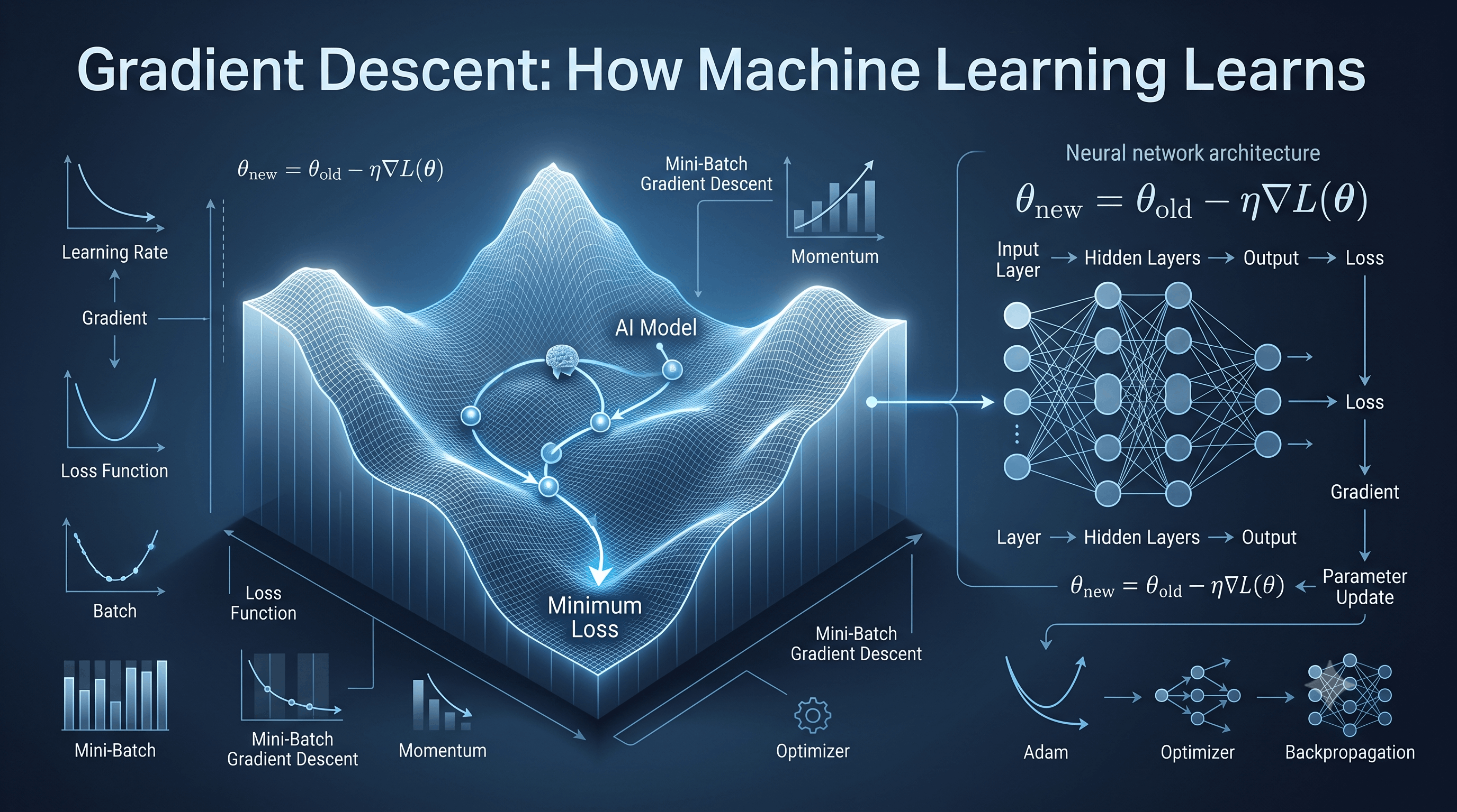
Gradient Descent is an optimization algorithm that iteratively changes model parameters to minimize a loss function.
In simpler words:
The model makes predictions, measures how wrong they are, and adjusts its parameters to become less wrong.
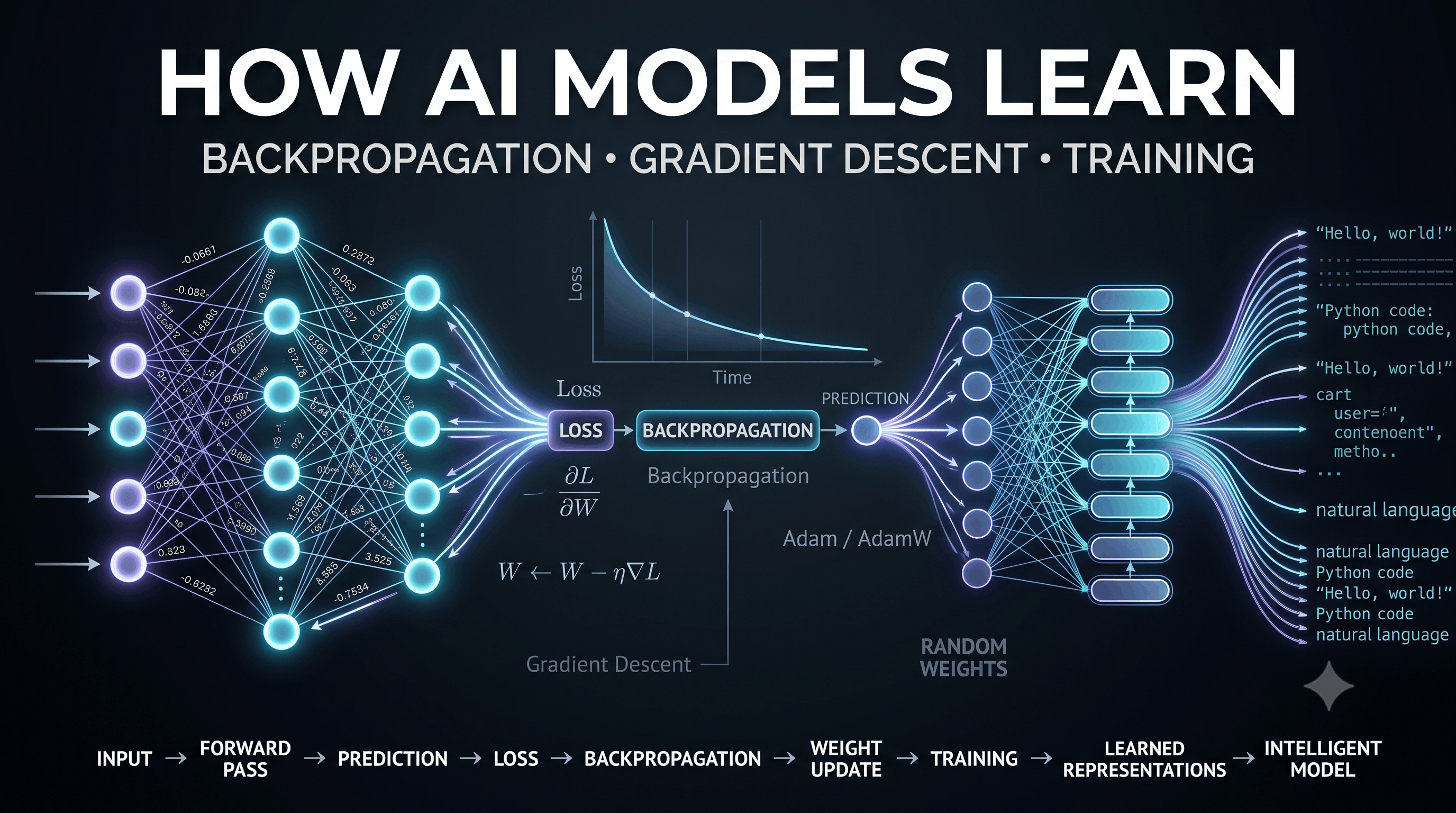
The basic process looks like:
Input Data
    ↓
Model
    ↓
Prediction
    ↓
Calculate Loss
    ↓
Calculate Gradient
    ↓
Update Parameters
    ↓
Repeat
This cycle can happen thousands or millions of times during training.
Imagine you're standing somewhere on a huge mountain.
You want to reach the lowest point in the valley.
But there's a problem:
You can't see the entire mountain.
You can only examine the slope immediately around you.
So you ask:
"Which direction goes downhill?"
Then you take a small step downhill.
You repeat:
Look at slope
     ↓
Take a step downhill
     ↓
Look again
     ↓
Take another step
     ↓
Repeat
Eventually, you may reach a low point.
That's the basic intuition behind Gradient Descent.
The mountain represents the loss function.
The horizontal dimensions represent model parameters.
The vertical dimension represents the amount of error.
For example:
Loss
 ↑
 │        ●
 │      /   \
 │    /       \
 │  ●           \
 │                ●
 │________________________→ Parameter
The goal is to find parameters that produce a low loss.
A loss function measures how far a model's prediction is from the desired answer.
Suppose you're predicting house prices.
Actual price:
₹50 lakh
Model prediction:
₹45 lakh
The prediction has an error.
A loss function converts that error into a numerical value.
For example, Mean Squared Error can be written as:
Loss = (Actual - Prediction)²
The larger the error, the larger the loss.
Without an objective, the model doesn't know what "better" means.
The loss function provides that signal.
Think of it as the model's scoreboard:
Prediction A
     ↓
Loss = 50

Prediction B
     ↓
Loss = 20
Prediction B is better according to this loss function.
Gradient Descent helps the model move toward parameter values that produce lower loss.
The gradient tells us how the loss changes with respect to the model's parameters.
For a single parameter:
Gradient = dLoss / dParameter
For many parameters, we have a vector of partial derivatives:
∇L(θ)
where:
L = lossθ = model parameters∇ = gradient operatorThe gradient points toward the direction of steepest increase of the function.
Therefore, Gradient Descent moves in the opposite direction.
The basic Gradient Descent update rule is:
θnew = θold - η ∇L(θ)
Where:
θ = model parameterη = learning rate∇L(θ) = gradient of the lossThe important part is:
-
We subtract the gradient because the gradient points toward increasing loss.
We want to move toward decreasing loss.
Imagine:
Current parameter = 10
Gradient = +2
Learning rate = 0.1
Then:
New parameter
= 10 - (0.1 × 2)
= 9.8
The parameter moves from:
10 → 9.8
Now imagine the gradient is:
-2
Then:
New parameter
= 10 - (0.1 × -2)
= 10.2
The negative gradient causes the parameter to move upward.
The algorithm is always trying to move downhill.
The learning rate determines how large each update is.
It is usually represented as:
η
For example:
η = 0.01
A small learning rate means:
Small steps
A large learning rate means:
Large steps
This seemingly simple parameter has enormous influence on training.
Suppose the learning rate is extremely small.
The model may make tiny updates:
Start
 ↓
tiny step
 ↓
tiny step
 ↓
tiny step
 ↓
tiny step
Training can become extremely slow.
The model may require a huge number of iterations to reach a good solution.
Now imagine the learning rate is huge.
The model might jump over the optimal region:
     ●
      \

        ●

              ●
Instead of smoothly approaching a minimum, the optimization can oscillate or even diverge.
We generally want a learning rate that is:
This is why learning-rate selection and scheduling are important parts of Machine Learning training.
Let's imagine a very simple function:
f(x) = x²
We want to minimize it.
The minimum occurs at:
x = 0
The derivative is:
f'(x) = 2x
Suppose:
x = 5
learning rate = 0.1
Gradient:
2 × 5 = 10
Update:
xnew = 5 - (0.1 × 10)
Therefore:
xnew = 4
Next iteration:
Gradient = 2 × 4 = 8

xnew = 4 - (0.1 × 8)

xnew = 3.2
Next:
3.2 → 2.56
Then:
2.56 → 2.048
The value gradually approaches:
0
That's Gradient Descent in its simplest form.
Now replace:
x
with:
Model Parameters
and replace:
f(x)
with:
Loss Function
Now you have the basic optimization process used to train many Machine Learning models.
Suppose our model is:
ŷ = wx + b
where:
w = weightb = biasx = inputŷ = predictionInitially, the model may have random or otherwise initialized parameters:
w = 0.2
b = 0.5
The model makes predictions.
Then we calculate the loss.
Next, we calculate how changing w and b would affect that loss.
Then we update them.
w → new w
b → new b
Repeat.
Eventually, the model can reach parameter values that produce much smaller error on the training objective.
Conceptually:
Initialize parameters

while not finished:

    Make predictions

    Calculate loss

    Calculate gradients

    Update parameters

return trained model
This loop is at the heart of many optimization-based learning systems.
In Batch Gradient Descent, the gradient is calculated using the entire training dataset for each update.
Suppose you have:
1,000,000 examples
The model may process all of them to calculate one gradient update.
Conceptually:
All Training Data
       ↓
Calculate Gradient
       ↓
Update Parameters
Stochastic Gradient Descent (SGD) updates the parameters using one training example at a time.
Instead of:
1,000,000 examples
       ↓
One update
you might have:
Example 1 → Update
Example 2 → Update
Example 3 → Update
...
The updates become much more frequent.
SGD can:
However, its updates are noisier.
Instead of smoothly moving downhill:
      ↓
      ↓
      ↓
      ↓
the path may look more like:
   ↘
     ↙
       ↘
      ↙
        ↘
Modern Machine Learning commonly uses Mini-Batch Gradient Descent.
Instead of using:
1 example
or:
Entire dataset
we use a small batch.
For example:
Batch Size = 32
The training process becomes:
32 examples
   ↓
Gradient
   ↓
Update

32 examples
   ↓
Gradient
   ↓
Update
And so on.
Mini-batches offer a practical compromise:
Batch Gradient Descent
        ↕
Mini-Batch Gradient Descent
        ↕
Stochastic Gradient Descent
They can:
These terms are often confused.
An epoch generally means one complete pass through the training dataset.
An iteration generally means one parameter update.
Suppose:
Dataset = 1,000 examples
Batch size = 100
Then approximately:
10 iterations = 1 epoch
So:
10 epochs = approximately 100 updates
assuming the dataset and batch structure remain unchanged.
Gradient Descent becomes especially important in neural networks.
Imagine:
Input
 ↓
Layer 1
 ↓
Layer 2
 ↓
Layer 3
 ↓
Output
Each layer contains parameters.
A large network might contain millions or billions of parameters.
The model needs to determine:
Which direction should each parameter move to reduce the loss?
This is where backpropagation becomes essential.
These concepts are related but not identical.
Calculates gradients of the loss with respect to the network's parameters efficiently using the chain rule.
Uses those gradients to update the parameters.
Think of it as:
Prediction
    ↓
Loss
    ↓
Backpropagation
    ↓
Gradients
    ↓
Optimizer
    ↓
Parameter Updates
So:
Backpropagation calculates the information needed for the update; the optimizer uses that information to change the parameters.
Gradient Descent is a basic optimization strategy.
In practice, Machine Learning often uses more sophisticated optimizers.
Examples include:
These methods modify how parameter updates are calculated.
Imagine pushing a ball downhill.
Instead of responding only to the current slope, the ball has some momentum from its previous movement.
Momentum-based optimization uses a similar idea.
It incorporates information from previous gradients to help the optimizer move more consistently.
Conceptually:
Current Gradient
       +
Previous Movement
       ↓
New Update
This can help accelerate training in useful directions and reduce some oscillations.
Adam stands for Adaptive Moment Estimation.
It combines ideas related to momentum and adaptive learning rates.
Adam maintains running estimates related to:
This allows different parameters to receive adaptive updates.
Adam became extremely popular in Deep Learning because it often provides a convenient and effective starting point for optimization.
AdamW is a widely used variant of Adam that handles weight decay in a way that is decoupled from the adaptive gradient update.
It is commonly used in modern neural network training.
For many modern Deep Learning workloads, AdamW is an important optimizer to know.
One common concern with optimization is the possibility of reaching a local minimum.
Imagine:
       \      /
        \    /
         \__/
           \
            \____
The model may reach a low point that isn't the absolute lowest point of the entire landscape.
In simple optimization problems, this can be a major concern.
However, neural-network loss landscapes are high-dimensional and more complicated, and practical training behavior is not adequately described by the simplistic idea that training always gets trapped in bad local minima.
A saddle point is a point where the gradient can be small or zero but the point isn't a local minimum.
A simple analogy is a mountain pass.
        /\
       /  \
------    ------
       \  /
        \/
Optimization can slow around such regions.
In high-dimensional neural networks, saddle points can be more relevant than the simplistic "local minimum trap" story often taught to beginners.
In deep networks, gradients can sometimes become extremely small as they propagate backward.
Conceptually:
Layer 10 → tiny gradient
Layer 9  → smaller
Layer 8  → smaller
...
Layer 1  → almost zero
If gradients become too small, early layers may learn extremely slowly.
This is known as the vanishing gradient problem.
The opposite can also happen.
Gradients can become extremely large.
Gradient
   ↓
10
100
1,000
100,000
Large gradients can cause unstable parameter updates.
This is known as the exploding gradient problem.
One technique used to address exploding gradients is gradient clipping.
For example, gradients may be constrained so that their magnitude does not exceed a predefined limit.
Conceptually:
Original Gradient
       ↓
Too Large
       ↓
Clip
       ↓
Controlled Gradient
This is especially common in some neural-network and sequence-model training scenarios.
The learning rate doesn't always have to remain constant.
A training process might start with:
Learning Rate = 0.001
and gradually change it.
For example:
Epoch 1   → 0.001
Epoch 10  → 0.0008
Epoch 20  → 0.0005
Epoch 50  → 0.0001
This can allow:
Large-ish steps initially
        ↓
Smaller steps later
Learning-rate schedules are widely used in Deep Learning.
Some modern training systems begin with a very small learning rate and gradually increase it before reaching the main learning rate.
This is called learning-rate warmup.
Conceptually:
Small LR
   ↓
Gradually increase
   ↓
Target LR
   ↓
Training
Warmup can improve training stability in some large-scale neural-network workloads.
Remember the previous article about overfitting?
Gradient Descent itself isn't the same thing as overfitting.
Gradient Descent is an optimization method.
Overfitting describes poor generalization.
However, how you optimize a model—including training duration, regularization, learning rate, and optimizer choices—can influence generalization.
For example:
Training continues
       ↓
Training loss decreases
       ↓
Validation loss eventually increases
This can indicate overfitting.
Suppose the loss function is:
Total Loss =
Prediction Loss
+
Regularization Penalty
The optimizer then tries to minimize this combined objective.
For example:
Loss
  +
λ × Regularization
where λ controls the strength of the regularization term.
This allows optimization and regularization to work together.
Let's put everything together.
             Training Data
                   ↓
             Neural Network
                   ↓
               Prediction
                   ↓
               Loss Function
                   ↓
             Calculate Gradients
                   ↓
              Backpropagation
                   ↓
                Optimizer
                   ↓
           Update Parameters
                   ↓
             Next Mini-Batch
                   ↓
                 Repeat
After many iterations:
Parameters
     ↓
Better Predictions
     ↓
Lower Training Loss
The model has learned parameters that perform well according to its training objective.
Here's a conceptual implementation of Gradient Descent for:
f(x) = x²
x = 10 learning_rate = 0.1

for step in range(50):
    gradient = 2 * x
    x = x - learning_rate * gradient

print(x)
The value of x moves toward:
0
because 0 minimizes:
x²
This tiny example captures the fundamental idea behind a much larger optimization process.
Imagine training a model to recognize cats and dogs.
The model begins with parameters that produce poor predictions.
Prediction:
Cat → 40%
Dog → 60%
Suppose the correct label is:
Cat
The loss is calculated.
Backpropagation determines how each parameter contributed to that loss.
The optimizer updates the parameters.
After many training steps:
Cat → 96%
Dog → 4%
The process repeats across millions of examples.
That is what we mean when we say:
The neural network learns from data.
Gradient Descent is an optimization algorithm.
It isn't the prediction model itself.
For example:
Linear Regression
+
Gradient Descent
can be used together.
Loss tells you:
How wrong is the model?
Gradient tells you:
How should the parameters change to reduce that loss?
They are related but different.
Not necessarily.
You should also examine validation performance.
Training Loss ↓
Validation Loss ↑
may indicate overfitting.
A large learning rate can cause unstable optimization.
Training may become unnecessarily slow.
Gradient Descent is a method that repeatedly adjusts model parameters in a direction that reduces prediction error.
It provides a practical way to optimize the parameters of many Machine Learning and Deep Learning models.
A gradient describes how a function changes with respect to its parameters. It points toward the direction of greatest increase.
Because the gradient points toward increasing loss. Subtracting it moves the parameters toward lower loss.
The learning rate controls how large each parameter update is.
Training may oscillate, become unstable, or fail to converge.
Training can become very slow and may require many iterations.
Stochastic Gradient Descent updates parameters using individual training examples, while the term SGD is also commonly used more broadly for stochastic or mini-batch-based gradient optimization.
It computes updates using a small subset of training examples at a time.
No. Backpropagation efficiently computes gradients; an optimizer such as Gradient Descent or Adam uses those gradients to update parameters.
Adam can be easier and faster to train with in many Deep Learning problems, but "better" depends on the task, architecture, data, and training setup.
If Machine Learning is about learning patterns from data, Gradient Descent is one of the mechanisms that makes that learning possible.
The basic idea is surprisingly simple:
Make Prediction
      ↓
Measure Error
      ↓
Find Direction of Improvement
      ↓
Take a Step
      ↓
Repeat
Millions of these small mathematical adjustments can transform an initially untrained model into a powerful predictor.
And this idea scales far beyond simple equations.
The same fundamental optimization concepts are involved when training modern neural networks with millions or billions of parameters.
But there's still one major piece missing.
We know that the model needs parameters.
We know Gradient Descent updates them.
But how does a neural network calculate those gradients through multiple layers?
That's where the Chain Rule and Backpropagation enter the picture.
Pixels to Perfection Design that Impresses